This job of witnesses � be carried out near
group TERA
ofthe universit� of the studies of Turin, and local
section INFN. Plan TERA
(YOUrapia with Radiazione Todronica) came promoted in 1991 with the scope to
carry in Italy new effective techniques of x-ray with uses of light
protons, Ionian neutrons and. Section INFN of Turin
participates to collaboration TERA with several attivit�:
It has cured the planning and realization of a dosimetro
three-dimensional, called magical cube
for the fast measure of the profile of dose deposited from
a therapeutic bundle.
It has developed codes for the drawing up of plans of
treatment with adroniche particles.
It has developed codes of simulation montecarlo to the low
energies like instrument of verification of the treatment plans or
like instrument of aid to the realization of the dosimetro
three-dimensional.
It has contributed to develop and it uses the code of
simulation GEANT4 in the within of controls on equipment radiological
hospitals worker.
It has contributed to searches on the cellular survival as
a result of radiation.
The contribution of the thesis � be that one to improve
and to carry the program for the drawing up of plans of treatment from
a language procedures-oriented (FORTRAN) to a language Object-Oriented
(C++). Such passage has the scope to align the code towards it
puts into effect them guideline in the computing and to reorganize it
second dictates me of the Object Oriented Programming (structuring of
the information and effective modularizzazione of the code). For
how much it concerns the improvement � instead proposed a new
algorithm for the calculation of the fluenze and opened the program to
the reading of two new ones form you of rows CT (Computerized
Tomograph): that CART, used from the machine for the TAC of
center IRCC
(Institute for the Search and the
Cure of Cancer) of Candiolo and that DICOM (standard much common one
for the exchange of medical images).
In understood it the 1 they come described the processes of interaction of the
cancellation with the matter that are inherent to the x-ray.
They come therefore described some biological aspects of this
type of interaction.
In understood it the 2 information equip on the x-ray leaving from the main
radioterapiche largenesses until arriving to modalit� of planning and
the release of dose to the patient.
In understood it the 3 the classes are described and the objects prepare to you
in order to support the constituent ones of the problem of the
calculation of a treatment plan.
Nel understood it 4 comes before introduced delle the procedures that
goddesses will make use methods and delle described classes nel third
party understood it (that relative to located sources a lot dal
target), beyond alla description far away detailed del program is
illustrates also turns out to you with it obtained to you.
Thankses
Ringrazio Teresa and my mother in order to have
to me supported for the job of which this thesis she represents the
final part.
Ringrazio moreover all the compagni/colleghi with which I have
divided these last months etc..
Understood it 1 Physical bases, biological chemistries and of the
x-ray
The passage of endowed particles of mass or
photons through the matter provokes, as a result of electromagnetic or
nuclear interactions, release of energy and physical mutations
chemical to the inside of the same matter. In an organism, such
mutations, can induce physiological alterations cio� modifications of
the operation of the cellular members, the cells and the entire
organism. The arc of acquaintances necessary in order to
re-unite cause-effect spaces perci� from the interaction
cancellation-matter to the reactions chemistries connected until the
biological and physiological answer of the organism. The main
slight knowledge necessary will come here of continuation taken in
consideration in order to cover, not too much in detail, such arc of
acquaintances.
1,1 Interaction of the cancellation
with the matter
The cancellations [1] are distinguished in two groups:
Directly ionizzanti cancellations:
composed from particles loaded that yield their
energy ionizzando or exciting atoms and molecules with the matter
through electromagnetic processes.
Indirectly ionizzanti cancellations:
composed from neutral particles and photons that yield all or
leave of the own energy to directly ionizzanti secondary particles,
which to they time, dissipates the energy cos� acquired exciting and
ionizzando the matter.
The greater part of the interaction between particles
loaded and characterized material � from electromagnetic processes
which had to the interaction between the electromagnetic field with
the particle incident and that one of electrons and the atomic nuclei
of the means in which one moves. A part smaller (but pi� always
important to the high energies) of the interaction � instead that
responsible nuclear of the fragmentation of the nuclei and therefore
of the tails of the peaks of Bragg (paragraph 1.1.1). As far as the
electromagnetic part they are distinguished:
Inelastic coulomb collisions with electrons of means.
Elastic coulomb collisions with the nuclei of means.
First they involve continuous loss of energy from part of
the particle incident through ionization and excitation of means.
The electrons emitted from the ionization process have initially
great kinetic energies and are therefore to they time ionizzanti
particles said
beams d :
in practical
they are the responsibles of the division of the energy lost from the
primary particle in means. The elastic collisions, viceversa,
give place to changes of direction of the motion of project them but
without appreciable losses of energy. The effect increases with
diminishing of the mass of the particle incident and &#"Calling
ghostscript to convert zImages/fig5.EPSF to zImages/fig5.EPSF.gif,
please wait..." 233; therefore particularly important for
particles to read (electrons) that hitting against the nuclei of the
matter they come diffuse to great angles also much, changing direction
abruptly and emitting consequently cancellation of braking.
This various dynamics in the collisions suggests to separate
the study of particles loaded to read (to electrons) from that one of
heavy particles loaded (those having greater mass with that one with the electron).
Release of energy
One defines stopping power
[2]
the valor medium of the loss of energy for unit�
of distance. It depends on the velocit� and from it loads
linearly with the ionizzante particle let alone () from the densit�
of crossed means. In a biological context one prefers however
to use the LET
(Linear andnergy Transfer)
that it represents the same
one quantit� but in the fixed water cio� to densit� r = 1 GM/cm3 and that measure usually in keV/ mm.
An other measure of the loss of energy the much common �
refraining power massico
that eliminates the
dependency from the average dividend the stopping power for the
densit� of same means (usually expresses in [ (MeVcm2)/(GM) ]).
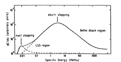
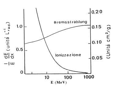
The loss of energy of heavy particles loaded �
caused from the Coulomb interaction with electrons with atoms target
(electron stopping)
or with theirs upgrades them nuclear (nuclear stopping).
The own ranges of energy of these two processes are
indicate to you in fig.
1.1.
Figures 1.1: Schematic Rappresentazione of the
processes of loss of energy for a heavy loaded particle.
Pu� to notice itself that to low energies the nuclear
predominates stopping while for all the other energies � the electron
stopping that cause the loss of energy. The intensit� of the
interaction it depends on the velocit� and from it loads. In
the case of the Ionian ones however it must consider loads average effective
which
depends in its turn on the velocit�. The electrons of project
having them velocit� an orbital minor of that one of project them
come in fact tear to you via in the collisions, consequently the
remaining electron number, and therefore it loads effective, are
function of the velocit� of projects them. To velocit� medium
many elevated all the electrons can be removed and it loads with the
ione equals its atomic number. With decreasing of velocit�
electrons they come captures to you from the material target and it
loads effective with projects diminishes them. It loads
effective � expressed from the formula empiricist of Barkas [2]:
ZEFF
= Zprt
(|
1 - exp(-125 bztrg2/3 )
)
"Calling ghostscript to convert
zImages/fig11.EPSF to zImages/fig11.EPSF.gif, please wait..."
"Calling ghostscript to convert zImages/fig10.EPSF to
zImages/fig10.EPSF.gif, please wait..."
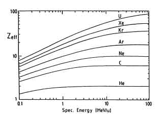
In fig 1,2
they are illustrates the values to you of ZEFF in
function of
the specific energy (energy for unit� of atomic mass; usually
expressed in MeV/u) of the particle it projects them.
Figures 1.2: It second loads effective the formula
with Barkas in function of the specific energy.
Pu� to notice itself that for 10 greater specific
energies of MeV all and the
six electrons of carbon
are it tears to you via.
The region of the nuclear stopping although to high biological effectiveness in how much the
nuclei can be bounces to you outside from the own molecular ties and,
in the fattispecie, also from the DNA, it does not turn out however
meaningful because it only happens to lowest energies and in limited
regions of space. The region ofthe
electron stopping � instead that one whose
biological effects are predominant and comes described from the
formula of Bethe-Bloch:
dE
dx
=
4 pand22ZEFF Nztrg
mandv2
ln
mv2
The 0ztrg
+ rel. terms
where
and
� it loads with the
electron
N
� the densit� atomic of
the target
ztrg
� the atomic number of atoms of the target
mand
� the mass of the electron
v
� the velocit� of the
particle it projects them
ZEFF
� loads effective with projects them
The 0
� it
upgrades them of calculable
effective medium
ionization for Z > 1 with the
formula semiempiricist:
0= 16 Ztrg0,9eV;
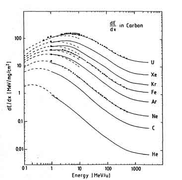
In fig. 1.3 come compare theoretical values (Bethe-Bloch) and
empiricists to you of the loss of energy (to be able refraining
massico) in function of the specific energy and
from the particle incident:
Figures 1.3: Comparazione between the loss of energy
measured with that theoretical in function of the specific energy.
Pu� to notice itself that the maximum release of energy,
as an example of Ionian carbon
� to
approximately 9 MeVcm2/mg equivalents to a 900
LET of KeV/mm
and that the same LET pu�
to be obtained to muovendosi different specific energies to two sides
of the maximum; to this same LET, tu"Calling ghostscript to
convert zImages/fig9.EPSF to zImages/fig9.EPSF.gif, please wait..."
ttavia biological effectiveness corresponds different: this
means that the same LET in if not � a complete parameter for the
determination of the biological effectiveness.
Range
From the curves of loss of energy (dE/dx) the quantit� can be obtained inverse (dx/dE) and, for integration on all the rilasciabile energy,
the range that the particle covers to the inside of means:
R =
. .
And0
0
dx
dE
dE
Being
dE/dx "a medium"
value also R it turns out to have a dispersion
s that it defines the
parameter of straggling to:
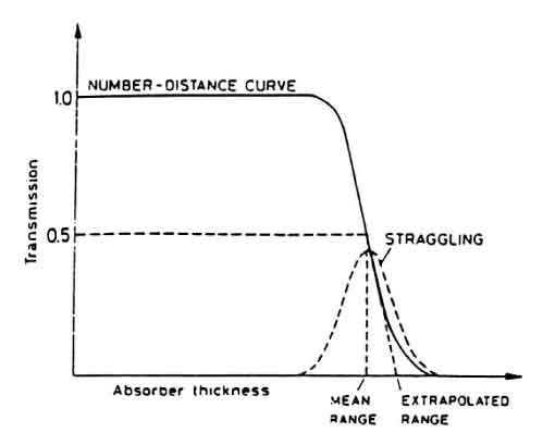
=.{2s}. In practical it comes
defined range medium
the distance for which the particle number begins
them � reduced of 50% and straggling the FWHM (Full Width Half Maximum) of the Gaussian one
that of it it represents the dispersion like pu� looking at itself in
fig. 1.4
where two curves
are represented: the integral curve that describes the course
of the still present particle number to one profondit� x and the
curve differentiates them that extension the particle number whose
equal way � to profondit� the x in abscissa.
Figures 1.4: Integral curve and differentiates them
of the heavy loaded particle distances in the matter.
The collected ranges calculate to you or measured they
come of usual in reperibili tables in literature, � however possible
to calculate the ranges for generic heavy particles taking advantage
of the fact that the fattorizzabile range � in terms of M (mass of
the particle), Z (loads) and one function only employee from the
velocit�
f(b):
Rp(b) =
Mp
Zp2
f(b)
Rx(b) =
Mx
Zx2
f(b)
Rx(b) =
zp2Mx
Zx2Mp
Rp(b)
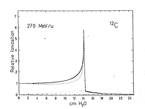
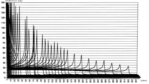
Peak of Bragg
Graficando the loss of energy of a heavy
particle loaded in function with the profondit� observes a plateu
that it leave from the take-off point in the material and arrives
until little cm from the range of the particle where begins to grow in
order then peaky whose width � of little milimeter which it follows a
second plateu with low values a lot pi� like pu� looking at itself
in figure 1.5
Figures 1.5: Densit� of ionization in
function of the profondit�. The outlined curve represents the
contribution goddesses nuclear fragments.
Such peak comes said peak of Bragg and its most remarkable therapeutic value for
first was intuito from Bob Wilson
which face to
notice in an article of last years ' 40 that used protons to
therapeutic scope would have interrupted theirs they traettoria on the
target without to provoke damages the rear woven ones. In the
fig. 1.5 famous a release
of energy also beyond the range: ci� � legacy to the fact
that the range only refers to the Ionian head physicians but exists
Ionian secondary (produced of reaction of the fragmentation) with
small atomic number pi� and therefore greater
range. The structure of the curves of Bragg pu�
to comprise itself on the base of the fig.
1.3: to high energies the
small warehouse of energy � and the particles continue in their
traettoria producing one densit� of low and almost constant
ionization; when the particles have been slowed down to 100
meaningfully inferior specific energies toMeV/u the
loss of energy grows quickly ulteriorly diminishing the velocit� in a
positive reaction that refrains the particle in little milimeter
catching up one LET
of proportions also 6:1
regarding the plateu of entrance.
1.1.2 Electron emission and
formation of the trace
For greater specific energies of 1MeV/u (region of electron stopping) the energy lost from the
head physicians � nearly totally transferred to electrons.
Based on the energy it begins them of the ione is had between
the 65-75% of the
rilasciata energy transformed in kinetic energy of electrons, 15-25% necessary for their
remaining ionization and the 5-15% come consumed in excitation electronic. In
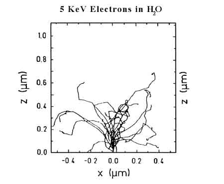
agreement to this distribution the greater part of electrons is freed
from their atomic ties and dissipates their kinetic energy to a sure
distance from primary collision (fig. 1,6) forming cos� a trace of
ionization around the traettoria of projects them.
Figures 1.6: Scattering of iniettati electrons to 5
keV in x= 0 0 in direction z.
The secondary electrons have
therefore scattering elastic and gasped to us. The scatter
elastic they do not dissipate energy practically but they determine
the angular distribution of electrons; those you gasped to us
go distinguished in energy: To low energies ( and
< the 20 eV ) secondary electrons do not
generate ionization practically but they are limited to excite atoms
of the crossed material. To greater energies it dominates
instead the ionization and such release of "Calling ghostscript to
convert zImages/fig3.EPSF to zImages/fig3.EPSF.gif, please wait..."
"Calling ghostscript to convert zImages/fig4.EPSF to
zImages/fig4.EPSF.gif, please wait..." energy has a maximum between
the 70 and the 200 keV, for
this reason highly energetic electrons become mainly reatti to you to
biological level (where they count the ionizations) when they come
slows down to you to energies of little hundreds of eV. The
transferred medium energy in the events of widely independent
ionization � from the energy of electrons and is worth between the 15
and 20 eV.
The combination of the transport and the release of energy of
electrons concurs with Montecarlo codes to
calculate with optimal verosimiglianza the traces left from Ionian in
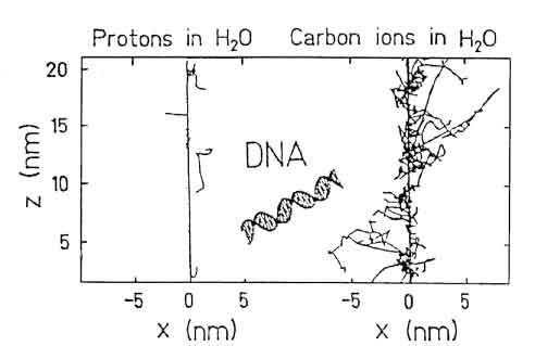
the matter. An example of such traces � illustrated in fig. 1.7 .
Figures 1.7: Comparazione between the traces of a
proton and one ione carbon
both with specific
energy of 1 MeV/u, in means � schematically
represented the structure of the DNA: ione the carbon produces
greater densit� of ionization causing damages pi� elevates you to
the DNA.
Online of principle the biological damage by means of the
comparazione of the structure of the trace with geometry of the DNA,
in practical would have to be possible predirre many efforts in such
direction has manifested the insufficiency of puts into effect them
capacit� of the computers in executing complex calculations cos�.
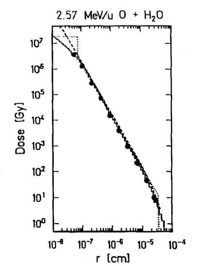
� be however evidenced, is to level experiences them that with
codes montecarlo course 1/r2 for the radial release of energy
of electrons around the trace, such turns out to you commonly is
accepted except for distances many small (hard-Core of high release of energy)
like indicated in fig. 1.8.
Figures 1.8: Radial distribution of the dose around
the trace of one particle: the dose decreases like 1/r2 on several
orders of magnitude of the radial distance.
The loss of energy differs from that one of heavy
loaded particles for two reasons: the fact that the electron
incident is identical to that one hit (that it
must be held in I compute in the quantistico calculation) and the fact
that the electron incident endures large shunting lines because of its
small mass (that it involves radiation for cancellation from loaded
particle braking bremsstrahlung).
The loss of energy is expressed perci� in two terms:
dE
dX
=
. .
dE
dX
. .
ion
+
. .
dE
dX
. .
brem
The first term is worth:
-
. .
dE
dX
. .
ion
=
2 p4andN
mandv2
r
. .
ln
. .
mandv2
2.2 I
. .
+
1
2
. .
for not relativistici electrons
(v < < c), and
-
. .
dE
dX
. .
ion
=
2 p4andN
mandv2
r
. .
ln
. .
2 mand g[ 3/2 ]v2
I
. .
-
1
2
ln (b) +
1
16
+
C
Z
-
d
2
. .
for relativistici electrons.
According to term it is worth:
-
. .
dE
dx
. .
brem
=
And
X0
where
1
X0
=
4Z(Z+1)NTo
137 To
rand2ln
183
Z1/3
with
rand=
and2
mandc2
beam classic of the electron. X0 � said length of cancellation
of
the crossed material and it represents the thickness of matter that
reduces, medium, the energy of the electron of a factor and:
< and > = and0and-x/X0
The loss of energy for bremsstrahlung grows
with the energy and becomes predominant to the high energies;
the relationship between the two losses of given energy �
gives
(dE/dx)brem
(dE/dx)ion
=
ZAnd
580 MeV
It is used to define, for every material, a
critical energy to of over of which the which had contribution to the
radiation becomes that one pi� large, such energy "Calling
ghostscript to convert zImages/fig6.EPSF to zImages/fig6.EPSF.gif,
please wait..." "Calling ghostscript to convert
zImages/fig7.EPSF to zImages/fig7.EPSF.gif, please wait..." pu� to
read to the intersection of the two curves illustrated in the fig. 1.9 and are worth:
Figures 1.9: Contributions of the two modalit� of
loss of electron energy in function of their energy.
Andc =
580
Z
MeV
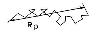
Because of the many shunting lines endured from
an electron in crossing means (fig. 1,10), � possible one not to properly define a completed
distance if in terms of medium distance of removal from the point it
does not begin them ( practical range ).
Its the following value �
described from formula semiempiricist:
Rp = 0,71 and1,72g/cm2
with and expressed in MeV.
Figures 1.10: Traettoria of an electron to the
inside of the matter and practical range.
Based on the energy and to crossed means i
beams X and g prime vary
types of processes: the more important are the photoelectric
effect, the Compton effect and the production of braces, except
important they are instead the coherent spread (or Rayleigh) and the
effect to fotonucleare.
Photoelectric effect
the
photoelectric effect consists in the collision between a photon and an
atom, with absorption of the photon and emission of an electron of
energy andand- equal to the difference between the energy of the photon
hn and the energy of tie of
the electron andb:
g+ To . To+ + and-
Andand- = andg - andb
The section of collision sf for photoelectric effect
depends on Z5 and has one equal energetic threshold to 300 keV.
For andb < < hn < < mandc2 and for electrons in shell the K of an atom with
atomic number Z the collision section can be used:
sph= 4.2sTto4Z5
. .
mandc2
hn
. .
[ 7/2 ]
where n it is the frequency of the photon, h the constant of
Planck, to
is the constant
of fine structure, sT the classic section of collision of Thomson(8pr2and/3), mand the
mass of electron and c the
speed of the light in the empty one.
The photoelectric process is dominant to the low energies
(hn <
0,5 MeV) and in the heavy
elements, for which he is still appreciable to energies of 4-5 MeV.
Effect Compton
Consiste in the
interaction between a photon and a free electron, on condition that
the energy of the photon is much greater one of the energy of tie of
the electron hn > > andb.
The expression analytics for the collision section isof Klein and Nishina:
sC=prand2
1
and
. .
. .
1-
2(and+1)
and2
. .
ln(2and+1) +
1
2
+
4
and
-
1
2(2and+1) 2
. .
with and = [
(hn)/(mandc2) ]
and rand the beam classic
of the electron.
The Compton effect dominates for energies comprised
between 0.8 and 4 MeV.
Creation of braces
Happens in the
coulomb field of a nucleus or an electron and consists in the
transformation of the energy of a photon in one brace
electron-positron.
For 1 < < [ (hn)/(mandc2) ] < < [ 1/(toZ[ 1/3 ]) ] the collision section
can be used:
s2andPC=rZ2
. .
28
9
ln
. .
2hn
mandc2
. .
-
218
27
. .
and for [ (hn)/(mandc2) ] > > [ 1/(toZ[ 1/3]) ], holding account of the
effect of screening:
s2andPC=rZ2
. .
28
9
ln
. .
183
Z[ 1/3 ]
. .
-
218
27
. .
The process happens for hn 3 mandc2 and is dominant for 5 advanced energies to MeV.
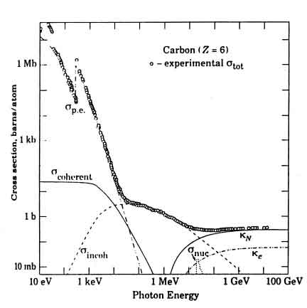
Section of collision total
To leave from the previous processes one can be
defined collision section total for the interaction of photons given
from the sum of the partial sections of collision:
Figures 1.11: Section of collision total and
contributions of the different processes for photons in carbon,
function of the energy ( sp.and.:effetto
photoelectric, scoherent: coherent spread, sincoherent: Compton spread, kn: production of braces in the
field nuclear, kand: production of braces in
the field of electrons, snuc: absorption to
fotonucleare)
The photon absorption
in
means has a esponenziale course and photon the N number that has not
endured interactions in a distance l is:
N=N0and-m�l
where N0 is the number begins them of
photons and the coefficient of linear
attenuation is defined like:
m = r
NTo
To
stot
with r density and To number of mass of the absorber; NTo is the number of
Avogadro.
The neutrons, do not equip you of load
electrical worker, they are not subject to coulomb interactions with
electrons and nuclei of the matter. They constitute however an
indirectly ionizzante cancellation because they interact with the
nuclei of the matter that cross through the force strong nuclear
producing ionizzanti particles. These reactions are rare events
in how much only happen when the neutron tos be distant less than 10-15m from the nucleus. The law
of attenuation of a thin monoenergetic neutron bundle � similar to
that one of the photons in the sense that come anch' they attenuates
to you through a coefficient of linear
attenuation esponenzialmente. The thermal neutrons ( and < 0,1 eV ) interact with the
atomic nuclei from which come "captured"; the nucleus then
diseccita emitting a photon. The probabilit� of neutronica
capture it increases diminishing of the energy of the neutron and
varies considerable to second of the absorbent material. The
section of great collision � for elements which the hydrogen, the
boron and the lithium. The fast neutrons (1 150 MeV < and < MeV) endure mainly hit elastic with
the nuclei, are worth to say that all the energy lost from the neutron
� transformed in kinetic energy of the nucleus ("moderation" of
neutrons). The maximum transfer of energy is had when the
frontal collision � and the nucleus have pi� or less the same mass
of the neutron, cio� when the target � a proton. Since rich
the biological hydrogen woven one �, the fast neutron passage in
characterized it � in greatest part from this type of interaction
that produces to protons of bounce of equal energy to that one of the
neutron incident, which cause to ionization and excitation in atoms
and molecules of means. Other damages to the living woven one
are caused from the collisions of neutrons with the nuclei of carbon,
oxygen and nitrogen.
Neutrons of intermediate energy interact by means of both
processes, of capture and elastic collision.
Others two interactions to remember are hit to it gasped to us and it hits to it
not-elastic. In the
first neutron it comes later on captured from the nucleus and riemesso
with one smaller energy and production of a photon. This
process single verification if the neutron has one at least energy of
1 MeV, necessary to excite the nucleus. It hits not-elastic
differ from previous because after the neutronica capture the issued
particle not � the neutron but a loaded particle. These
collisions have place for 5 advanced energies to MeV and theirs
probabilit� to take place itself grow to increasing of the energy.
Finally, for neutrons with advanced energy to 100 MeV pu� to
have the spallazione
,
cio� the fragmentation of the nucleus hit in pi� parts.
1,2 Reactions consequent
biological chemistries and to the ionization
The ionizzanti cancellations produce to the
inside of the matter ionizzati atoms and molecules or excite to you.
From the moment that an organism living � compostoi to the 70-85% of water [the 3] probable processes pi�
happen on it:
(radiolisi)
H2Or
cancellation
\leadsto
H2Or++and-
(excitation)
(excitation) H2Or
cancellation
\leadsto
H2Or*
The three species, H2Or+, H2Or* and and- they are diffused in following
means and gives to place phenomena:
H2Or++H2Or. H3Or++OH?font >
H2Or*.
. . .
. .
H2Or++and-
H?font >+OH?font >
H2+Or?font >
"Calling ghostscript to convert
zImages/elsolvat.EPSF to zImages/elsolvat.EPSF.gif, please wait..."
The electron produced from H2+Or?font >, once slowed down, is arranged to the center of four
water molecules takes the watery electron name
and constitutes one chemical
species much reactive. One its particular reaction �:
H2Or+andaq-. H2Or-
Also the molecule H2Or- (like H2Or+) � unstable:
H2Or-. H?font >+OH-
After ~ 10-11sec from the passage of
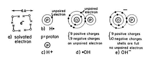
the ionizzante cancellation four remain chemically active species H3Or+,OH?font >,H?font > and andaq-.
(fig. 1,12)
Of which:
H3Or+ + and-aq . H?font >+H2Or
They remain perc� the following free
radicalses: OH?font >:
ossidrile radical H?font > : radical hydrogen andaq: watery electron
Such radicals are many reagents you since also being
electronically neutral they stretch to couple the electron spaiato
with an other similar one of an other radical, or to eliminate the
electron with a transfer process. Moreover they can interact
with organic molecules RH (where R is members of the molecule and H a
hydrogen atom) forming radical secondary:
Figures 1.12: Species reactive produced in the
radiolisi of the water: to) watery or solvatato electron andaq-,
b) radical H hydrogen?font >, c) ione hydrogen H+, d) radical idrossile OH?font
>, and) ione idrossile OH-.
RH+OH?FONT >. R?font >+H2Or
RH+H?font >. R?font >+H2
Both these free radicalses (primary or
secondary) can interact with biologically meaningful molecules
provoking the so-called
indirect radiobiologico
damage.
Pi� very rarely has viceversa a
directed radiobiologico damage when organic
molecules RH endure the direct action of the cancellation.
RH
cancellation
\leadsto
RH++and-. R?font >+H++and-
The free radicalses interact also with oxygen
molecules originating other harmful free radicalses; in oxygen
presence an increase of the consequent biological damage to the
cancellation passage is had thereforeeffect
oxygen.
Or2+H?font >. I HAVE2?font >
Or2+and-. Or2-
Or2-+H+. I HAVE2?font >
Moreover oxygen pu� also to interact with other
free radicalses:
The nucleus of the cell � demonstrated
sensitive hundred of times pi� to the attack of the produced free
radicalses from the cancellation passage.
Such
radicals are not moved very from the place in which they have been
produced because of their elevated one reattivit�, if they react with
the DNA wants therefore to say that they have been produced in its
grip prossimit�. The damages that can provoke are following:
Cancellation of one base (Bd: base deletion): a base is removed from the nucleotide;
Alteration of a sugar (Knows: sugar alteration):
change of the property chemistries of the
desossiribosio;
Alteration of one base (Ba: base alteration): change of the property chemistries of one organic
base (To, T, G or C);
Erroneous pairing of base (Mb: mismatched base): it comes altered the natural connection between
bases A-T and G-C.
Breach of chain (Sb: strand break): breach of the covalent bond between the sugar
desossiribosio and the groups phosphate;
The outcome of the damages produced to the DNA
regarding the life of the cell depends on the phase of the cellular
cycle in which they they take part ( G1 maturation of cell,quite G0,S synthesis of new chromosomic material,G2 preparation to the mitosis,M mitosis) and from the
capacit� of the same cell to repair just the genome. In any
case there are of proteins sensors that find following the endured damage and send one of
the three marks them cellular:
arrest of the cellular cycle
apoptosi
repair
Arrest of the cellular cycle
the cellular cycle comes interdetto and in such a way the
capacit� is stayed out of duplication of the cells.
Apoptosi
This process determines
the dead women cellular without however priming typical inflammatory
processes of the necrosis, this � in fact the genetically programmed
way of cellular suicide to the aim to guarantee the organism renews of
its cells.
Repair
If one of two sides of the
double propeller of the DNA comes characterized like "wrong" one able
protein � of risintetizzarlo for "complement" to the integral
considered opposite side. This process of repair pu� not to
prime itself if a double breach of chain
(DSB double strand break) in this
case is had in fact the repairing protein does
not succeed to carry a.termine its job.
The DSB just defer therefore from the SB (single strand
break) because they cannot be repairs to you, this � the reason for
which cancellations to elevated densit� of ionization (high LET),
which they have greater probabilit� to realize two near damages
between they (fig. 2,2)
biologically turn out pi� destructive (or effective in the perspective of the
x-ray).
One first measure of the quantit� of
cancellation absorbed from woven � a densit� of energy medium and rilasciata from
ionizzanti particles in one infinitesimal mass rdV tending to zero [4]
D=
lim dV. 0
and
rdV
In International Sistema its unit of measure � [Jkg-1] which it comes given the name of Gray[Gy] . A submultiple
of the Gy � rad= 10-2Gy.
Equivalent dose
In radioprotezione (than it is distinguished
from the x-ray for the low dealt doses) uses the equivalent largeness dose that
holds account of the harmfulness of every detailed list cancellation
by means of a factor of weight for the
cancellationwr. The equivalent dose in a woven given T � from
the expression:
HT=
. r=cancellation
wrDT,r
Its unit of measure in International Sistema
would be anch' it the Gray but in order to remember that it is
multiplied for a factor of adimensional weightwr
it takes the name of Sievert [ Sv ].
Effective dose
In the within of the radioprotezione account
also of the greater or smaller sensibility to the cancellation from
part of woven through a factor
of weight
for woven w the Twith T an index of the woven one
is always kept. A largeness is obtained that it serves to
giving to an esteem of the damage total endured from an individual as a result of one exposure to
cancellation:
And=
. WovenT=
wTHT
RBE
In the x-ray viceversa (high doses) the
"harmfulness" of the type of cancellation takes to the name of
"effectiveness" understanding as ability to bring damage to the cells.
In order to quantify it one is used relative measure making
reference to one very precise cancellation champion (indicated with
the pedice g ):
biological effectiveness
(RBE
, Relative Biological Effectiveness
is defined relative) the expression:
RBEr=
Dg
Dr
Where Dg is the dose necessary in order to
produce the same damage produced from the D doser of
an other cancellation (indicated with the pedice r ). (If D
r) then RBE=2 is necessary the double quantity ofdoseof conventional cancellation(Dg = 2). In
practical it is used to directly put in relation the value of the RBE
with the LET
(gi� defined in the first one
understood it but that verr� resumed in the next paragraph) of the
not conventional cancellation why it is fundamentalally on that the
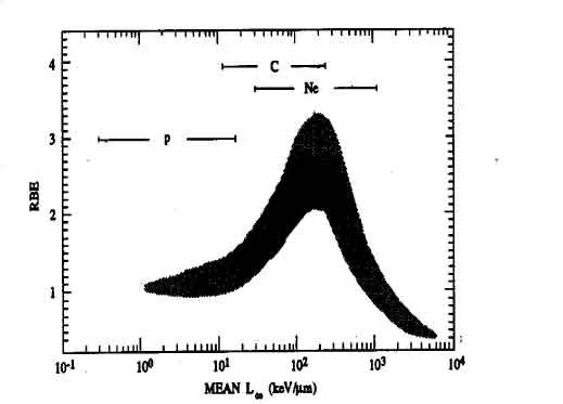
biological effectiveness of a cancellation depends. In fig. 2.1
Figures 2.1: Rappresentazione of the data
experiences them (obtained on several cellular lines) of the
dependency of the RBE from the LET. The segments p, C, Of it indicate the obtainable
LET with protons, Ionian carbon
and Ionian neons.
pu� to notice itself as to increasing of the LET there is
an increase of the RBE (since increases to the concentration of
ionization and therefore the probabilit� of a DSB
(double strand break: double breach of the
propeller of the DNA, not repairable); with the progressive one
to increase of the LET however has a sovrappi� of energy release
that, while it does not increase the damage diminishes however the
number of places in which such release it happens because of the
greater dissipation of energy.
LET
The amount of energy transferred from the
directly or indirectly ionizzante particle in the space unit
determines the distribution of the ionization and the excitations to
the inside of the biological material and harmfulness (RBE) of the
same cancellation. LET is defined (To delineate Energy
Transfer) the amount:
LET=
dE
dx
where dE it is the medium energy transferred to means from the
particle in covering a feature dx in its inside. In table
2,1
they are introduces the
values to you of the LET of the main cancellations used in x-ray [5]
Particle
It loads
Energia(MeV)
LET(keV/mm)
Electron
-1
0.01
2.3
0.1
0.42
1
0.25
Photon
0
1.17-1.33
0.2 2
(g of the 60Co )
Proton
+1
2
16
+2
8
+5
4
+10
0.4
to
+2
5
95
Neutron
0
5
3-30
Ione carbon C+6
6
10MeV/u
170
250MeV/u
14
Table 2.1: Ionizzanti LET of cancellations
and interesting particles in x-ray
In fig. 2.2 "Calling ghostscript to convert zImages/dna.EPSF to
zImages/dna.EPSF.gif, please wait..." "Calling ghostscript to
convert zImages/p13.EPSF to zImages/p13.EPSF.gif, please wait..."
"Calling ghostscript to convert zImages/t5.EPSF to
zImages/t5.EPSF.gif, please wait..." the dimensions of the traces of
several particles regarding those of the DNA can be confronted:
it is obvious as for particles to high LET (as the particle to in issue is one more
elevated possibility than double breach of the propeller of the
consequent DNA with greater biological effectiveness.
Figures 2.2: Schematic Rappresentazione of the DNA
and the traces of an electron and a particle to that they cross it.
OER
They exist you vary chemical factors that
influence the biological effect of the cancellations, between these
the main one is surethe effect oxygen . The molecular oxygen presence (Or2)
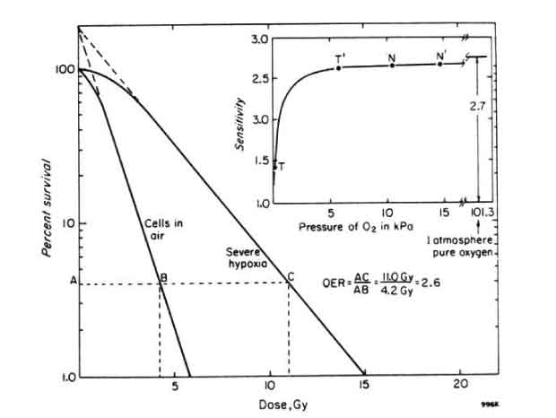
increases to a lot the damage endured from cells (fig. 2,3).
Figures 2.3: Of survival for cells irradiated in
presence or 2 Or percentage absence; with the
points To, B, C comes graphically illustrated the meant one of
quantit� the OER. The file illustrates the radiosensibilit� in
function of the partial pressure of Or2.
In order to obtain a determined biological effect in woven
devoid of oxygen (as the nucleus of a tumor) is necessary a dose of
greater cancellation poich� is less of the sensitive half to the
cancellations [6].
Viceversa in woven very oxygenates to you is sufficient one
smaller dose of cancellation. This ascertainment empiricist has
three explanations:
- the oxygen presence cause an increase of the production of
free radicalses.
- molecular oxygen has one elevated affinity electronic
and stretches therefore to react with electrons freed from the
ionization delaying some the recombination and increasing the
probability from part of the electron to cause damages.
- the oxygen lack between a radiation and the other of an
aliquot treatment diminish the ability to recovery from part of the
damaged cells.
Quantitatively the effect oxygen expresses through amount OER
(Oxigen Enhancement Ratio), defined as the relationship between the
demanded dose in order to bring a sure damage to one cell in ipossica
condition respect to one condition of normal oxygenation:
OER=
D
D0
Where D � the dose necessary in order to
produce to a woven effect in real and
0D � the dose that would
produce the same effect if the woven one completely were oxygenated in
air to normal pressure. In fig.
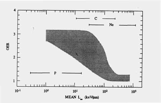
2.4
Figures 2.4: OER in function of the LET
for several types of cancellations and several lines cellulari.Sono
indicates the raggiungibili ranges to you of
LET
for interesting particles in x-ray.
it can be noticed like the several OER in function of the
LET.
The x-ray is used in order to destroy a
localized tumor facendogli to absorb one such dose of cancellations to kill of the
cells. Sometimes work also on the p"Calling ghostscript to
convert zImages/t3.EPSF to zImages/t3.EPSF.gif, please wait..."
"Calling ghostscript to convert zImages/t7.EPSF to
zImages/t7.EPSF.gif, please wait..." "Calling ghostscript to
convert zImages/doprofot.EPSF to zImages/doprofot.EPSF.gif, please
wait..." ossibili way of spread of the tumor in order to prevent that
proliferi elsewhere. Fundamental in both cases � the fact that
the tumorali cells turn out pi� vulnerable medium to the cancellation
of those knows some and this guarantees a space of job (in terms of
dose) muovendosi to the inside of which � possible to bring a fatal
damage to the bearable tumor but for the other cells. Such
stimabile space � from the curves dose-effect
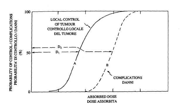
(fig. 2,5).
Figures 2.5: Curves dose-effect: (a) woven
tumorali (b) woven healthy. Therapeutic relationship is defined
quantit� the D2/D1 where 2D
and D1 is the
doses that have one probabilit� equal to 50% to provoke respective
complications the woven ones heal and control on the tumor.
In such figure pu� to observe itself that for a dose
correspondent to a probabilit� next to the 100% of control on the
tumor (line To) one is had also probabilit� a lot (too much) elevated
to obtain damages to the woven ones heals. For this reason the
radioterapista chooses of usual a such dose not to go up beyond 50% of
probabilit� of having damages on the woven ones heals, for as these
curves are introduced this mean also to have only 50% of probabilit�
of control of the tumor.
If however it is succeeded to having good selettivit� a ballistic one
or
conformit�
in the sense
that is succeeded to irradiate only the tumor nearly then (always
making reference the fig.
2.5) an only horizontal line is not had pi� represented the
absorbed dose but one brace of lines one for the dose absorbed from
the tumor (than far� reference to the curve (a)) and one for the
woven dose absorbed from healthy (that far� the reference to the
curve (b)).
With I use it of hadrons
is succeeded to
obtain an increase of probabilit� of cure of a tumor in how much the
dose absorbed � pi� concentrated in the tumorali woven ones of how
much is succeeded, viceversa to obtain with electrons or photons (this
for the gi� cited characteristic of the peak of Bragg
that resumptions will come later on however).
Initially the x-ray was practiced using like
sources of cancellation of the radioisotopi like cobalt, today it is
preferred to use linear electron accelerators which can produce
directly make us of monoenergetic electrons or (refraining electrons
on targets to high densit�) it makes us of photons characterizes you
from a continuous phantom of energies with energy maximum
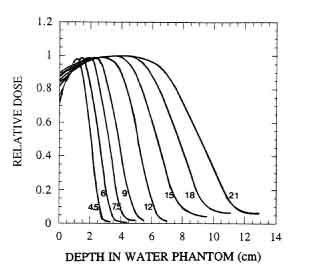
correspondent to that one of electrons. In figures 2,6 and 2,7 they are visualizes the
release to you of energy in photon and electron water respective.
Figures 2.6: Curves dose-profondit�
in water in order make us of electrons of energy comprised
between 4.5 and 21 MeV.
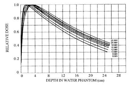
Figures 2.7: Curves dose-profondit�
in water in order make us of having photons the maximum
energies for energies comprised between 6 and 25 MeV.
Electrons
It makes us of electrons have the maximum
distance to the inside of the woven one (than � approximately equal
(in cm) to the met� of the energy begins expressed them in MeV), to
of l� of which one is had tail of lowland intensit� due to photons
of bremsstrahlung.
For this type of energy release the electrons are
adapted for the treatment of superficial tumors
or to the maximum to some centrimetro sottopelle.
Photons
It makes us of photons are viceversa
characterizes to you from an absorption of preceded decreasing
esponenziale type from a maximum that does not go beyond i 4 cm for
photons also several energetic (25 MeV).
Theirs I use particularly � indicated for "deep" tumors
situates you to many centimeters from the cute.
For irraggiare in selective way such targets they have been
developed technical sophisticated, that they imply the necessit� to
use pi� makes us that they enter in various points of the body but
that they are all focuses to you on the center of the tumor.
In order to realize this type of treatment it is necessary that
the entire linear electron accelerator wheels around a fixed point in
the space (isocentro)
so as to to be able to use
whichever take-off point of the bundle prestabilito regarding the
patient. A way in order "to conform" the bundle to the tumor �
moreover that one of frapporre of the obstacles between the source and
the target so as to to make to reach specific doses in every point of
this. In such sense today they are used of the "obstacles"
whose varied shape dynamically saving in time and costs of realization
respect the obsolete "obstacles" to fixed shape. Such dynamic
objects come call "multileaf collimators" (
collimators to you to many leaves) in how much are
constituted from parallelepipedi of heavy metal that move sliding on
the other for means of motors and frappongono to the bundle coming
true itself some the modulation in intensit�.
For adroterapia the x-ray practiced with
composed particles from quark agrees: neutrons, protons,
Ionian.
Neutrons
As far as neutrons, their release of energy in
water � much similar one to that one of photons and turns out
particularly useful single in how much the boron has the two following
propriet�:
1) fixed on some woven tumorali.
2) it interacts with thermal neutrons freeing particles to to high LET that
rilasciano locally all their energy.
Such propriet� they concur to realize the boroterapia that consists
exactly in making so that the boron fixed on the tumorale woven one in
issue which it comes then irradiated with thermal neutrons triggering
a reaction that free particles to that rilasciano dose exactly where such necessary dose
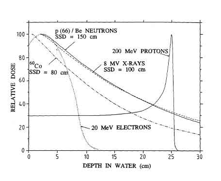
�. The release of energy for neutrons � visualized in fig.
2,8 with to that one of
electrons, photons and protons.
Figures 2.8: Curve dose-profondit� for photons, (da
one cobalt source and a linear accelerator from 8 MeV), neutrons and
protons. For every bundle source comes indicated the distance
"skin" ("Source to Skin Deep").
Protons
The curves dose-profondit� for protons
(2,8) di"Calling
ghostscript to convert zImages/t13.EPSF to zImages/t13.EPSF.gif,
please wait..." "Calling ghostscript to convert
zImages/t14.EPSF to zImages/t14.EPSF.gif, please wait..." fferiscono [7] strongly from those
of the other cancellations up to now analyzed in how much heavy
protons (and particles loaded) in a generalized manner rilasciano the
doses pi� elevated to the end with their distance in the woven ones
giving place to the "peak of examined Bragg" gi� in the first one
understood it. For protons therefore low the superficial dose
� regarding that one absorbed in the region of the peak, various from
how much succeeds for photons and neutrons.
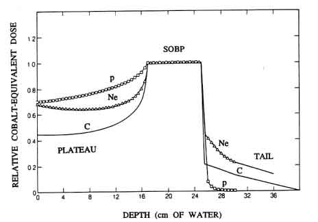
The profondit� of the peak of varied
Bragg with the energy it begins them of protons:
modulating it opportunely � possible to obtain plateu in the
said curve a dose-profondit� SOBP (Spread-out Bragg Peak; peak
of Bragg increased) illustrated in fig.
2.9.
Figures 2.9: Peak of increased Bragg (SOBP) in order
makes us of Ionian protons and.
With a plateu of this type a null release of dose beyond
the target is succeeded to practically avoid very many woven dose to
healthy (you �), however pu� to make oneself better still with
Ionian light in how much, like pu� noticing itself in fig.
2.9 the dose rilasciata before the low peak � a lot pi� as the
loaded particle becomes pi� heavy.
Ionian light
Ionian the light ones
concur therefore a good "conformation" of the dose even
if introduce the following problems:
1) to realize a complex accelerator of Ionian � pi� that to
realize of one for single protons.
2) as the mass of the ione increases introduces the phenomenon
of
the fragmentation
gi�
seen in the first one understood it that it provokes to the release of
dose also beyond the peak of Bragg (tails)
like
pu� looking at itself in fig. 2.9
. In practical it has single sense to use Ionian
not pi� heavy of oxygen.
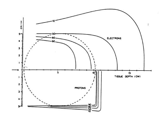
The greatest advantage to use the adroterapia in place of the
traditional therapy (photons, electrons) appears obvious in fig.
2.10,
Figures 2.10: Comparison between the
distributions of dose makes us of protons and electrons on a target
(represented from the circle).
in it it comes quantified the qualit� of the consistent
treatment obtained with a proton bundle increased comparing the curves
of isodose with those due to an electron bundle.
� seen as the hadrons offer the advantage of
a distribution of dose in profondit� with a pronounced maximum to the
end of the traettoria regarding the esponenziale deposition of photons
or the maximum a lot increased of electrons, in this way they concur a
conformazionale therapy
of elevated precision.
Such precision concurs to adapt the distribution of the dose to
the shape of the volume very well target, diminishing at the same time
the dose received from the woven ones you heal and saving the critical
organs us.
The plan of radioterapico treatment must be planned holding
account of a series of multidisciplinary parameters that go from the
diagnostic one, to the radiomedicina passing for the technological
limits and problematic relative biological physics and to the
modalit� of release of the dose.
In a generalized manner, schematically, we have following is
made:
Acquisition of diagnostic information (CT, PET, NMR,
others reperti).
Location of the volume target and the organs to risk
limitrofi.
Chosen of the doses and modalit� of release (the type of
x-ray, position of sources, eventual I use of collimators)
Elaboration of the treatment plan second one of
following modalit�:
direct planning
direct Appraisal of
the plan of treatment with method tries and tries again.
inverse planning
automatic
Elaboration of a plan of treatment through reversal
algorithms
.
Simulation and three-dimensional visualization of the
distribution of obtained dose.
The data of departure for the formulation of a
treatment plan are constituted from obtained diagnostic images with
various techniques. They in fact, beyond supplying means for
the appraisal from the clinical point of view of the extension and the
positioning of the lesion, contain also the relative information to
the three-dimensional anatomy of the patient. This last
information carries out the most important role in the drawing up of
the TP(Treatment Planning), since concurs to estimate the eventual
presence of organs and/or structures to risk in the vicinities of the
tumor, and to trace therefore the contours of the volume target and
those surrounding ones, beyond allowing the choice of the
characteristics of the bundle and opportune geometry of radiation
pi�.
The diagnostic images moreover contain also the relative
information to the distribution space them of the densit� to the
inside of the body of the patient, than, once converted in a map of
the powers refraining massici in water, � to the base of the
dosimetrici calculations for the drawing up of the TP.
E' important to emphasize the necessit� to decide of a set of
diagnostic images of the patient in the radiation position, in order
to arrange of a simulation of treatment pi� the possible supporter
with the realt�, suit of all the necessary data for the location of
the lesion and the positioning of the patient on the lettino or the
chair of treatment (clip surgical, signs tatua you on the skin, etc).
This last tied to the possibilit�, pi� always diffuse
requirement �, to obtain reconstructed radiografiche images to leave
from the diagnostic images of departure, that they can be compared
with of the x-rays carried out in knows it of treatment during
ciascuna therapy session, in order to guarantee an adequate one
riproducibilit� of the positioning of the patient.
The technique of the computerized tomography
� necessarily main the diagnostic source (example for pathologies to
the tiroide PET
1
does
not turn out pi� valid for the appraisal of the physiological state
of the same tiroide) however constitutes in the greater part of the
cases the source from which part in order to elaborate a treatment
plan, eventually coadiuvata from other sources of images which the PET
exactly or the NRM.
the 2
CT are based on the absorption of i beams X from part of
the crossed woven one, such absorption depends on the densit�
electronic of the material that constitutes the woven one and comes
measured from a coefficient, saying
coefficient
of absorption or linear
attenuation m. [8]
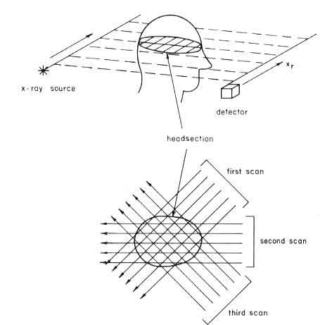
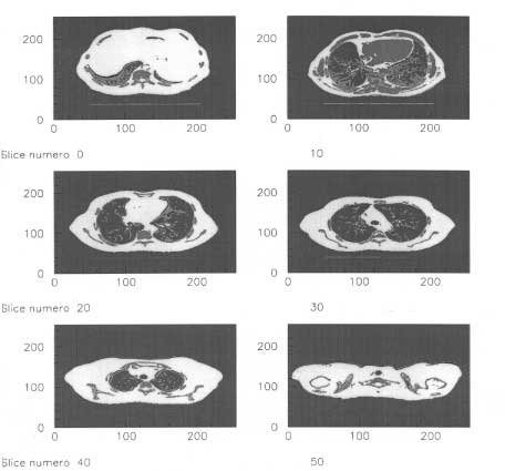
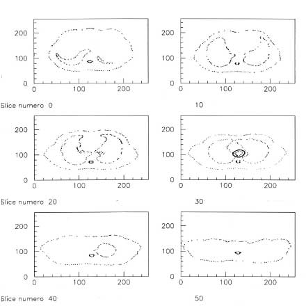
In order to realize the CT the orga"Calling
ghostscript to convert tac.EPSF to tac.EPSF.gif, please wait..." in
issue it does not come ideally subdivided in many slices
of limited thickness
(typically approximately a millimeter), ognuna of these comes
therefore sondata individually using makes us of beams X. (fig. 2,11)
Figures 2.11: System of scanning for
tomography. A bundle of beams X passes through the object and
comes revealed to the escape. The system (source of beams X -
detector) up slides along the directions indicated in the figure
(scansion). Pi� scansions comes carried out to several angles
for being able to better reconstruct the image of the organ.
To every scansion it comes measured the curve of
absorption of the cancellation in function of the position of the
system source-detector. The information of all are always
collected therefore the scansions (of the same one slowly) and through
algorithms sosfisticati enough laughed them in way pi� or less
precise to the densit� electronic in every point of the woven one.
(the precision increases with the number of scansions but ognuna
of they it brings a damage upgrades them to the patient in how much
rilascia dose to the woven ones for which not pu� eccedere)[9]. In rough but pi�
perhaps intuitiva one way much pu� to say that
from the analysis of the "ombre/trasparenze" seen from
pi� angles-shot pu� to reconstruct the forma/densit� of the object
in examination.
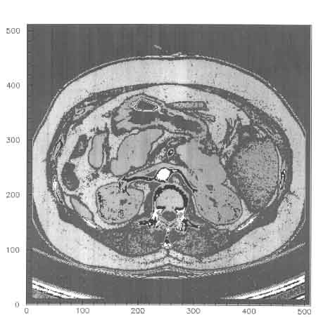
The elaborated differences of
densit� cos� are such to concur the distinction between woven and an
other nonch' � eventual pathology of same weaving. It must
per� specify that of fact, through the scansion technique the
coefficients of absorption m can only be measured (k,and) where
k it represents the identificativo of a particular one voxel and and
the energy of i beams X uses you. In order to pass to the
densit� electronic
true and own it must
calibrate (through scansions to famous materials) the acquisition
system elaborating the coefficients that tie the densit� electronic
to the absorption coefficients:
rand=
(To +B�m)
. .
electrons
cm3
. .
In order to render pi� the data collected on the
absorption coefficients leggibili it is used per� to report them to
that difference-percentage regarding those of the water still
multiplies to you for 1000 for magnificarne the difference [10], such values take to the
name of number of Hounsfield
or
number TC:
TC(k,and) =
m(k,and) -mH2Or
mH2Or
�1000
L"Calling ghostscript to convert hu.eps to hu.gif,
please wait..." "Calling ghostscript to convert
zImages/a246.EPSF to zImages/a246.EPSF.gif, please wait..." to
relation between densit� electronic and numbers of Hounsfield differs
regarding that one with in coefficients of absorption only for the
coefficients that normally come expressed in the following shape:
rand=
(To +B�10-3�TC)�1023
. .
electrons
cm3
. .
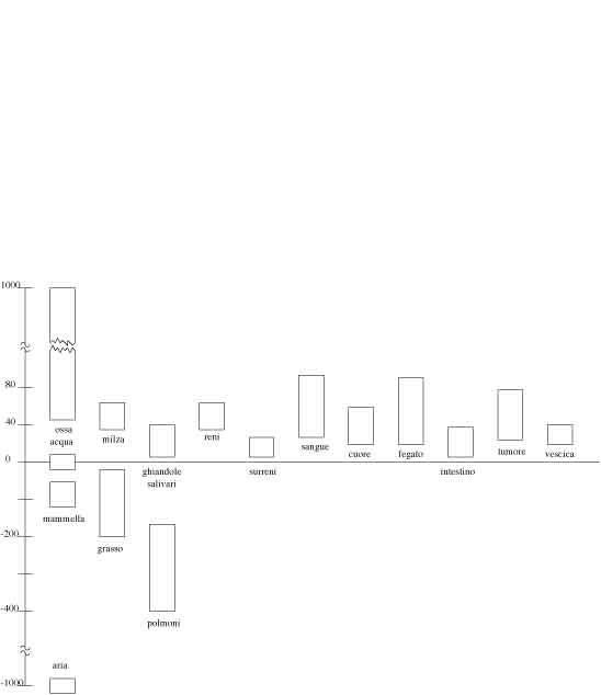
From the definition of number of Hounsfield it is observed
that for air TC=-1000, while for water
TC= 0. The values of woven
numbers TC for the several one of the human body are reassumed in
figure
2.12.
Figures 2.12: Distribution of woven numbers TC for
the several one of the human body.
A tie between densit� electronic exists finally rand and
densit� of the material:
Making reference to the images of the woven one
to cure the doctor it supplies its prescription as far as the dose
that in it goes rilasciata.
Knowing a priori the impossibilit� to only localize the dose
on the tumor and knowing moreover the limits of
the equipment to disposition in order to realize the treatment, the
doctor supplies one demanded of dose release that is reasonably
obtainable.
Such demand comes represented with of the curves of isodose
(cio� contours long which the dose assumes constant value) traced
directly on the image of the woven one. With sophisticated
systems pi�, viceversa the doctor pu� to take advantage itself of
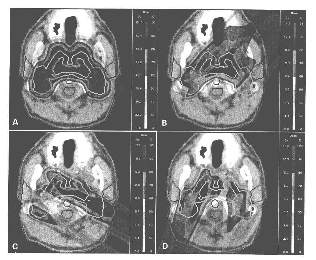
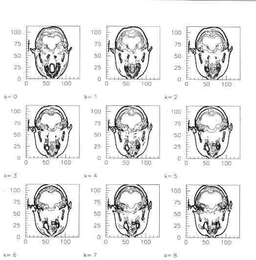
the aid of a computer for stilare a treatment plan. In fig.2.13
Figures 2.13: Curves of isodose for
treatment with protons to intensit� modulated.
� possible to see one shielded of one of these programs
for the elaboration of treatment plans: up on the left the
curves of isodose turning out from the complete treatment with 9 are
observed make us of protons. E' important to emphasize that the
optimization of the physical
distribution
of the dose does not coincide with the
optimization of the treatment plan, because the influenced
radiobiologico effect � from other parameters, which the division
outline and the radiosensibilit� cellular. In order to judge
the effects of the radiation � therefore always necessary to estimate
also
probabilit� of control of tumor(TPC)
and probabilit� of damages to tessuuti normal (the NTPC) noticeable from the reading of the curves the
dose-effetto"Calling ghostscript to convert magn.EPSF to
magn.EPSF.gif, please wait..." "Calling ghostscript to convert
rascan.EPSF to rascan.EPSF.gif, please wait..." for the woven ones in
issue.
For somministrare a consistent dose on a tumor,
the method better � that one than a modulation in intensit� of the
bundle by means of bolus
cio� obstacles frapposti between the source and the
target (does not arrange of passive distribution
of the bundle) but by means of dispositi in a
position to generating it makes us to you of various energies
(arranges of active distribution of the
bundle).
Using of disposed magnets on the distance of the bundle
� moreover possible to modify of its direzione.(fig. 2.14
Figures 2.14: Schematic structure of a
system to magnetic scansion.
With the union of the two modulations � possible, in the
case of the adroterapia to center the peak of Bragg in very precise
points of the volume to deal executing of one three-dimensional
scansion [11].
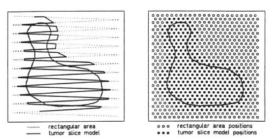
Such scansion pu� to be of two types: raster or voxel
(fig. 2,15).
Figures 2.15: Systems of scansion: to) raster b) voxel.
With the method raster the continuous bundle � and moves to zig-zag, with the
method voxel the
intermittent bundle � and situates the peak of Bragg to the inside of
a small volume that pu� to be also of the order of the millimeter of
side realizing therefore a treatment extremely
in compliance with the same tumor.
The program must be in a position to supplying a
treatment plan
that consists in with of spot
described gives: particle direction,
number, energy. Such slowly of treatment it must be elaborated
to leave from the following things:
from the CT that describes the organs to deal
from the prescription of the doctor on the parts
to deal and with which doses
from the description of the equipment that
effettuer� the treatment and from the positioning of the patient
regarding the bundle
From the program it wants moreover the
visualization of the doses that with the plan of elaborated treatment
is previewed comes rilasciate (necessarily not identical to those
prescribed); such doses will have, in phase of verification,
being convalidate with simulations montecarlo or experience them.
Detention remaining these objects the program to you has
however many degrees of libert� that they follow evolversi of the
situation, as an example:
In version ANCOD2 � decided to accept like format CT only
standard DICOM
realizing of the converters to this
format in order to integrate form owners to you gi� deals to you in
the previous version of the program coming from from the following
centers:
PSI (Paul Scherrer Institut Switzerland),
GSI (Gesellschaft fur SchwerIonenforschung Germany), Molinette
Hospital (Turin), Hospital IRCC of Candiolo (Institute Search and the
Cure del Cancer, Turin);
The prescription of the doctor on the parts to deal comes
supplied in a format owner of the program in attended of one deepened
study pi� of standard DICOM;
The description of the equipment that effettuer� the
treatment is limited currently to the position of the source and as an
example does not hold tie account eventual on the energies available;
The program pu� to work with Ionian carbon or protons:
in order to extend it to other particles it must supply ulterior
tables of data on the energy release.
Respect to a language procedures-oriented where
the concentrated attention � on the flow of events that door from a
set of data in input towards a set of data in output [12] in a language
object-oriented is attempted more rather than to characterize the
single ones entit� that they concur to constitute an informative context considering
the procedures as contingent events
whose
plasticit� and facilit� of realization they are guaranteed just from
a good disarticulation of 13 same data[] Every member of the
informative context from which wants to extract information must be
rendered independent as far as the creation, maintenance and callback.
These componenti("Oggetti")
must be able
to be exchanged between several the modules of the procedures without
that there is other code that sovraintenda to ci�: a matrix
must contain in if its number of elements and the module pu� calmly
to recall it without preoccuparsi to try information to its care
elsewhere.
This formulation demands taken care of a study of the
informative context but code drawing up concurs one once pi� snella
that this � be placed in system.
A ' other characteristic of 14 languages
object-oriented[] �
that one to concur the creation of new "types" of data.
As an example if the program makes algebra use to
delineate convene to create a new type of data, in this case "matrix"
and to define for it sum operations, multiplication, reversal etc, so
that the code can contain instruction of the type
To = B + C; To = B * C;
Where To,B,C are matrices.
The introduction of new types facilitates therefore very many
the code drawing up and must be used every time is a reasonable one
probabilit� of res-use in the same informative context [15]. In the drawing up of
treatment plans as an example the study of the trajectories of
particles, of the appraisal of the distances etc, suggests to the
creation of objects which geometric points, lines and plans with
relati algorithms to you for the calculation of the intersections, the
distances and quant' other.
With of a entit�
logically very delineated, joined to the algorithms that them are own,
it constitutes one "class". As an example in this program � be
introduced the Rijk class that concurs the management of matrices of
real numbers with 3 indices (creazione/inizializzazione, destruction,
access, visualization, memorization on rows, callback from rows, it
prints).
All the informative context pu� to be structured on pi�
levels: they introduce entit�/tipi base in order then to
define complex others entit� pi� that of it make use.
The important, in the drawing up of the informative
context, � to characterize the hierarchical levels in which well it
structure. Such location � tutt' stable other that univoca or:
� work of the project manager to estimate how much time to
spend in the study of the architecture and when and how much to modify
it to unexpected forehead: a vision to sgrossamento begins them
continuation from successive approximations seems to be one good road
[13] or however � be
that continuation in the drawing up of this program.
Here of continuation they will come described,
to leave low from pi� the hierarchical level, the classes that
constitute the informative context which procedure ANCOD2 far�
reference in the elaboration of the treatment plan.
The hierarchy of the classes � following:
Level -1: REALdef
Level 0: SystemOfUnits Int3Vector Hep3Vector
Level 1: Linens GridBox
Level 2: Rijk R1R1 RiRjR1
Level 3: PAW RUN (ReadDICOM, findFluence, readDataCard,
findEnDeposited, ReadRange, others...)
For being able to proceed in the reading �
per� opportune to open a short parenthesis on the C++ that concurs
one understanding, even also only highly summarized, of its main
constituent ones.
The instruction #
includes
The structure of a C++ program � following:
# it includes < iostream.h > int main(){int i; cout
< < `` Inserire a number ``; cin > > i; cout < < `` inserted
Number = '' < < i; return 0; }
This program carries out a input from keyboard
(cin = console
input) and a output on c
finishes them (cout =onsole
output).
You notice that the first instruction ( # includes < iostream.h >) that
of fact substitute from a precompiler with
the content of the rows comes iostream.h
says the
compiler that verr� made use of a set of instructions that they
concern input and output through operating of stream
(< < and > >);
operating whose meant evince from the same example. This
particular � a lot important , in fact the C++ compiler comes conceived like opened: removed a nucleus
able base to carry out the elementary operations pi� the rest of the
compiler comes integrated from many modules of which some they are present standards
of the C++ in every compiler, others is own of the specific
compiler and, above all it previews that good
part of the added modules will have been created
from the same programmatore. This characteristic, joined to
others potenzialit� of the base nucleus that we will see later on,
concurs the programming Object Oriented. The functions
One good rule of programming � following: you divide and conquest:
the sum of the difficolt� of a problem divided in two � in
fact from the human point of view much minor of that one of the same
problem considered in its together. In order to succeed to
divide a problem the "functions" are used where, for function not only
something agrees that gives back to a number but also something that
it carries out of the operations.
Here of
continuation it comes brought back the example of declaration of a function ("min")
in order to find the minor between two numbers and its I use:
int min(int to, int b) {/* Declaration */if(to < b) return
to; if(b < to) return b; } # it includes < iostream.h >
int main() {int i,j; cout < < "To insert two numbers"; cin
> > the > > j; cout < < "smaller Number =" < < min(i, j);
/ * I use */return 0; }
The rows header and implementation
In the previous example declaration
int min(int to, int b)
implementazione
if(to < b) return to; if(b < to) return b;
and I use
cout < < "smaller Number =" < < min(i, j);
of the function min they were all and three in same rows whose name could be
as an example "prova.cc". Normally instead these three parts
come subdivided in how much
The declaration must be
present in every program that utilizzer� the function min: in it the function and the
type of since are described to the type of data given back from every
argument represents (in this case all int). The declarations become
part in rows with suffisso h that it takes the name of header rows in how much, like for < iostream.h >, porr� a # is included with its name in head to the rows that far� I use some. rows min.h:
int min(int to, int b);
The implementazione
must be
present in rows with suffisso
cc of which eseguir� the compilation obtaining itself rows
with suffisso o that
through the linker of it
consentir� I use it from part of whichever program that utilizzer�
the function min. rows min.cc:
# it includes "min.h" int min(int to, int b){if(to < b)
return to; if(b < to) return b; }
In order to obtain the rows with suffisso o of
this program dovr� giving the following commando:
cxx - c utilizzo.cc
(you notice yourself that with the instruction # it includes "min.h"
in
these rows, declarations of the function are had of fact two "min":
ci� it guarantees that who writes the implementazione does not
confuse some type of data in fact if the two equal declarations are
this do not constitute problem but if they are various the compilation
it interrupts and it comes marked an error.)
I use the program that uses the new function of the
called C++ min dovr� to
have the following structure:
rows
utilizzo.cc:
# it includes "min.h"/* Callback of the definition */#
includes < iostream.h > int main() {int i,j; cout < < "To insert
two numbers"; cin > > the > > j; cout < < "smaller Number
=" < < min(i, j); / * I use */return 0; }
In order to obtain the rows eseguibile (with
suffisso exe) of this program dovr� giving the following commando:
cxx - c min.cc - or min.exe min.o
Where the last term (min.o) means that it comes
executed
link (a connection)
to the module previously compiled (min.cc)
so as
to to be able to use the function min().
The classes
Beyond to the functions they can be defined of the classes that are of
the given structures that they have of the
methods that of it concur the manipulation.
Example of a class could be that one of the complex numbers:
a complex number � composed from a brace of real numbers for
which � defined the sum, the product, the difference and the
relationship. The sintassi in order to create a such class,
however, � of all the banal one and does not introduce one here class
a lot pi� simple.
rows unaClasse.h:
class unaClasse{private: int to; public:
void set_a(int num); int get_a(); }
# it includes "unaClasse.h" # includes < iostream.h > int
main(){unaClasse var1; unaClasse var2; var1.set_a(10);
var2.set_a(22); cout < < var1.get_a(); cout < <

var2.get_a(); return 0}
This program, once compiled and executed
produrr� the press of numbers 10 and 22.
For ulterior deepenings on the C++ one sends back specific
witnesses of which some titles them they are indicates to you in
bibliography.
This module defines a priori (for this � be
placed to "level -1") what agrees for "real number": I use of double guarantees greater
precision and velocit� of execution, that one of "float", viceversa,
one smaller memory requirement.
All the classes to follow definiranno REAL the real numbers,
where replaced REAL verr� from double or float
to
second of how much content in this module.
This module � be ritagliato from bookcases
CLHEP (CLasses for High Energy Physics) [17]
coming from from the
CERN and consists in one series of definitions of constanti. In
it the definitions of unit� of measure in terms of multiples and the
submultiples of a chosen value as fundamental and equal place to 1 are
contained.
Es. for the lengths we have the following definitions:
With this definition � therefore possible to use
instructions like:
thickOfDetector = 5*mm;
or (using the definitions of the energies):
enOfParticle = 5*MeV;
All this avoids of having to bring back to part the
conventions on the unit� of measure assumed and turns out very
chiarificativo in the reading of other people's code.
This class serves for being able to manage
like one only entit� one tern of indices. Examples of I use
are the gunlayer to particular voxel, a gunlayer that it in its turn
constitutes the index of an element of the matrix containing densit�
electronic of all the voxel.
The first instruction declares and inizializza the
variable one spotVoxel.
The second one uses the implicit initialization in the sense
that being does not specify you the values of the single members these
comes settate to zero from the constructor.
it prints
:Questo method ( < < )suggerisce to the compiler as the
press of a type data must be carried out int3Vector:
comparison: This
method concurs to confront between they two int3Vector:
/ * (actualSpot and spotVoxel they are two int3Vector)
*/flagEqual = false; if (actualSpot=spotVoxel) flagEqual = true;
These instructions settano one variable logic to second of
the equality or less of the two int3Vector. (Two int3Vector they
come obviously defined equal if they have all and the three equal
members).
As it suggests the name this class comes from
bookcases CLHEP from which per� � be enucleata and reduced.
The phase of installation and I use of bookcases CLHEP in fact
has introduced a such series of problems to suggest to send back to
the future its completion, this also in virt� of the fact that the
program would have used a part however much limiting of the same
bookcases. Of the CLHEP � remained the sintassi of the
constructor and the methods it implements (cio� those to you that
have not been excluded) so as to to guarantee of a compatibilit�
tomorrow. The class � the not entire but real version of the class int3Vector,
servants cio� as an example to manage terns of real numbers (useful
for the carriers in the space or generic "three-dimensional" data).
constructors: two possible
ways exist to create a Hep3Vector (to
istanziare); in which the members come
inizializzate to a value (zero if not explicitly supplied) and an
other in which the members come copied from an existing Hep3Vector
gi�.
set the methods setX(),setY(),setZ()
assign the values of the members x,y and z of the carrier;
the behavior � of all the analogous one to that one of the
methods setI(), setJ(), setK() of the class int3Vector that pu� to
look at itself like example to pag. pageref.
get: the methods of
withdrawal of money x(),y(),z() give back the values of the
members x,y and z of the carrier; also here the exemplified
behavior � in the methods int3Vector to pag. pageref.
comparison: the operating
ones == and! = they give back the logical value
true if two int3Vector they are
respective equal or various, viceversa give back the value false.
distance
the method distance(B) supplies the distance
between the variable one of Hep3Vector type that of ago use and
variable (anch' it of type Hep3Vector) B. (Second the conventions adopted in SystemOfUnits the expressed distance
sar� in milimeter).
int3Vector A=(0.0,0.0,0.0); int3Vector
B=(3.0,0.0,0.0); cout < < "the distance between" < < To < <
"and" < < B < < "is worth" < < A.distance(b);
These will produce on the video the written one:
The distance between (0.0,0.0,0.0) and (1.0,1.0,1.0) is
worth 1.0
The class Linens � be realized to the aim to represent a
particle bundle that leaves (or passes) from a point and directs
towards an other point. (Pi� that of a line draft in realt�
of a oriented line) the
methods of intersection with the orthogonal plans to the aces is
concurred therefore to evidence the traettoria of one particle.
constructor
In order to define a
line comes given respective to the point of arrival (p1) and the point
of departure (p0):
# he includes "Line.h" # includes "SystemOfUnits" #
includes "Hep3Vector" int main(){Hep3Vector p1(0.2*mm, 0.3*mm,
0.4*mm); Hep3Vector p0(1*m, 2*m, 3*m); Linens beam(p1,
p0); }
This program does not complete no operation
except that one to define a line that "leaves" from the point p0 and
"it goes" to the point p1.
it prints
the press method
( < < ) produces in output the
two preceded constituent points the line from the words "from" and
"to":
/ * (Direction of the beam is beam the declared line in
the previous example) */cout < < ": "< < beam;
It produces on the video the written one:
Direction of the beam: from (0.2,0.3,0.4) to
(1000,2000,3000)
(you notice yourself that the values of the
coordinates have been prints all to you in milimeter)
intersections with plans
the methods intersectionPlaneX(xx),
intersectionPlaneY(yy), intersectionPlaneX(zz) give back the coordinates of the point of intersection
between the line that recall them and the flat X,Y or Z (orthogonal
respective to axis x y and z of the system of reference) indicated
from argument xx, yy and zz.
In "plane" future it could turn out useful to define a class and
to realize a method of generic intersection with (a slowly not
necessarily orthogonal one to the aces of the coordinates as it
happens currently).
This class serves in order to manage a reticulum of plans that it
characterizes with of parallelepidi that sayings come buckets, box
or voxel.
In practical every element pertaining to this class pu� to
visualize like one "three-dimensional shelf": what it counts
they are not the contents to the inside of the buckets but the
dimensions and the number of the same buckets. The class only
supplies therefore geometric indications but it returns very useful in the identification
and the management of the typical volumes of the treatment plans:
TTV (TorTto Volume) and the PTV (Pwools of Treatment Volume).
Every voxel it has a center center and one left
inferior chine
node, later
on comprender� the importance of such distinction.
(they define left inferior and
advanced right the points with pi� and pi� respective great small
algebriche coordinates).
constructors
have been implement
two methods to you of construction of a data of GridBox type:
The first method has like arguments rispettivamento x0,y0,z0 coordinated of the left "inferior" chine, follows therefore
three braces of data that represent the number of voxel and their long
dimension every axis.
According to method it serves to identify a sottovolume
whose left inferior chine (origin) coincides with a sure node of the volume "parent" (in
this case node (21,20,19)) and whose dimension in terms of number of
voxel comes supplied like third party and last argument.
it prints
the method ( < < ) produces R-in.stampa information
on the origin, the number of voxel and their dimension of a data of
GridBox type:
Origin: (1000, -80, -80) Number of Voxels: [
52,50,49 ] Voxel dimensions: (3,3,3)
origin
the method origin() gives back to a
data of containing Hep3Vector type the coordinates of the left
"inferior" angle of the "GridBox" (those that are visualized in the
press previous to right of the word "Origin").
dimensions of voxel
the method dimensions() give back to a
data of containing type int3Vector the number of voxel along every
direction. Applying to this data the method of withdrawal of
money of the members just of the data of type int3Vector � possible
to extract one particular dimension:
GridBox TTV(100*cm, -8*cm, -8*cm, 52, 3*mm, 50, 3*mm, 49,
3*mm); cout < < "Number of long Voxel Y =" < <
TTV.dimensions().i()
Produrr� R-in.stampa
Number of long Voxel Y = 50
left inferior chine (of all grid)
the method lowerCorner() gives back the coordinates of the origin (considered the
chine with small algebriche coordinates pi�.)
skillful advanced chine (of all grid)
the method higherCorner() gives back the coordinates of the antipoidale point to the
origin regarding the center of the GridBox, in practical the point
with great algebriche coordinates pi�.
With of these two last methods it allows to estimate the
"measures of I block" of the GridBox and comes as an example used from
the same class in order to estimate if a determined geometric point
makes part or less of the Gridbox.
position of the center of voxel
a
method centerPosition gives
back a Hep3Vector that represents the geometric coordinates of the
center of determining voxel. Two possible calls to this function
exist (what in C++ it comes called polimorfismo):
int3Vector spotINDEX(1,2,3); Hep3Vector spotPOINT;
spotPOINT = TTV.centerPosition(spotINDEX); / * before
called */Hep3Vector firstSpotPOINT; firstspotPOINT =
TTV.centerPosition(4,4,4);/* second call */
The first call has like argument a type data
int3Vector while the second one has like argument three entire.
Although it can be made less or of one or of other before turns
out useful when for some reason in the present an index to three
members and not program � gi� wants scinderlo, the second one turns
out viceversa useful when as an example they make to slide indices i
singularly, j, k and a carrier to 3 indices is not wanted to be
recomposed.
position of a chine of voxel
a
similar method nodePosition() � del all (also for how much regards
the polimorfismo degli arguments) al method centerPosition() but
center gives back to the coordinates dello left inferior chine del
voxel rather than those del.
belongings to grid
the method include(P) give back second
a true or false value booleano that to the geometric coordinate P (a
Hep3Vector) are found less or to the inside of the GridBox structure.
An example of I use verr� given with to the next method.
from space coordinate them . index voxel
the method insideWhichVoxel(P) has like
argument one geometric coordinate (a Hep3Vector: P) and gives
back a tern of indices that represent the voxel to the inside of which
the P point is found. The function � planned in order to give
back a number, such number would not have sense if the point is not found to the inside of the
GridBox: this method must therefore be used in concomitanza with
that one includes:
GridBox TTV(100*cm, -8*cm, -8*cm, 52, 3*mm, 50, 3*mm, 49,
3*mm); Hep3Vector P(100.1*cm, -8.1*cm, -8.1*cm);
if(TTV.include(P)){cout < < "the P point resides in the voxel" <
< TTV.insideWhichVoxel(P)}
These instructions produrrano following prints:
The P point resides in voxel [ the 0,0,0 ]
In how much the control of
belongings to the GridBox � be verified.
In fortran [18] I use it of matrices to 2 or pi� indices �
defined in definitive way univoca and from the standards of the
language. In C++ it comes supplied I use analogous that does
not turn out per� much efficient one in how much historically derived
from the C with a system
of gunlayer gunlayers that turns out slow in approaching the data.
Moreover the C did not have methods, they did not exist
therefore operating of press or manipulation of the matrices that were
not of the functions to part. For who it wants to use matrices,
or also only carriers, in C++ � therefore advised to reperire of
package gi� ready (� the case of the CLHEP or
the Standards Template Library (STL)
[19] or to rewrite itself of the
classes optimizing them for just the type of I use. In ANCOD2,
as an example, to part the reversal does not appear elements of matrix
algebra and the matrices are fundamentalally of the containers to
three indices of numbers of Hounsfield, densit� electronic or other:
from here the creation of the Rijk class.
The methods of the Rijk class are:
constructors, the Rijk class
possesses three costruttori:uno express
(without initialization), one with
initialization and one copy from one given Rijk matrix gi�:
The first three arguments constitute the names of the three dimensions and
are useful in case it is decided to use the same class in order
memorizzare always given to three indices but whose meant it could as
an example be various ( r, q, f if the matrix contains elements whose geometry �
that one of a field of spherical segment.
Second the three arguments represent in long number of elements
the three dimensions.
it prints This method ( < < ) prints all the entrances of
the matrix; if the matrix � much large one convene to use the
methods
showInformations() and store() that
they supply only some information respective one and a press on rows
the other. Such methods will come later on however described.
it prints propriet� the method showInformations prints the
names of the three dimensions and the long number of elements ognuna
of they; it turns out particularly useful in order as an example
to verify if the callback of a matrix from rows (Rijk_Restore) � gone to good aim
or if viceversa the matrix in issue has of the various dimensions from
that we expected.
dimensions are five functions of
withdrawal of money of the dimensions:
sizeI(), sizeJ(), sizeK(), sizeIJ(), sizeIJK
Where sizeIJ() and sizeIJK() they are respective the number
of elements in one slide (constantK=) and total.
names
Others three functions serve
to capture the names of the three dimensions:
nameI() nameJ() nameK()
set
the method put(i, j, k, value) concurs of
settare the value of one entered of the matrix.
get Esistono Two functions of withdrawal of money of one
entered:
get(i, j, k) and
get([ (ijk)\vec ])
Both give back a type data "double".
memorization and callback from rows
the methods store(nomefile)
and
Rijk_restore(nomefile)
serve in order memorizzare and to recall from rows one
matrix; their use � following
It restores the matrix from rows. This
mechanism pu� to be useful as an example in order memorizzare
matrices the whose elaboration � be expensive and sar� always the
same one, rather than ricalcolar it every time therefore memorizza
once calculated and the obtained result is red-use later on. It
is advised to use rows with suffisso "a Rijk" in order to identify of
pi� the contents easy.
The matrix comes
memorizzata in the rows in ASCII (cio� with alphabetical characters)
former for slide and with correspondence of lines and columns
respective with the first one and according to index (and j).
Such choice, coadiuvata with a editor able to manage lines
without length limits (as xemacs ) or with a system of press to many
columns like a2ps [21]
, allows to
a direct comparison of one image of CT with the read numerical values
(slide for slide). As an example a matrix whose entered they
are:
The data are written in written
ASCII with ulterior added that they concur to give of an
interpretation also for who eventually wanted as an example to read
them from a program written in FORTRAN. In the order
the meant one of the data and the written ones �:
- Names of the three dimensions
- Number of elements for every dimension
- Order with which they are memorizza you the data
- Pointer of slice new beginning (K =...)
- Lines of data
Visualization
the Rijk
class � moreover known from a module PAW.CC
that includes the following functions: PawPlot(Rijk), PawPlotAlongX(Rijk) , PawPlotAlongY(Rijk) that
creates of the histograms long three directions in order to visualize
of the contents of the matrix (Z � that one of default). The
module PAW.CC and the graphical visualization will come explain to you
later on.
A relation of type y=f(x) pu� to
be tabulata like with of values (xi,yi) if the famous
function not � or if its calculation turns out particularly heavy for
the calculating. This, as an example, � the case of the
En function(range) that alloy a set of specific
energies to the correspondents range (distance of the peak of Bragg in
water) for Ionian protons or carbon. Class R1R1 serves
therefore in order to manage a "relation" in mathematical sense
between two insiemi of real numbers calls Dom to you (for dominion)
and Img (for image). Important � that
the values of the dominion are given in increasing order, otherwise
some methods of the class will not work.
constructor
the constructor has
three arguments, the name of the dominion, the name of the image and
the number of braces of values:
R1R1 range("Range[mm]", "Energy[MeV/u]",47);
set the method put() concurs to insert the-but the
brace of values:
dimension
the method size() gives back a data of
entire type that represents the number of braces of values memorizza
you.
n-mo element in the dominion
the
method nthDom(i) gives back
the element of the dominion pertaining to the-but the brace of values.
n-mo element in the image
the
method nthImg(i) gives back
the element of the image pertaining to the-but the brace of values.
interpolation
the method linInterpolation(x0) linearly gives
back the value of y (image) interpolated between value y(xprec(x0)) and that one y(xsucc(x0)). If the great or
too much too much small value of x � regarding the range in which �
defined the relation an error comes marked.
previous element in the dominion
the method getDomLeftTo(x0) gives back the value in the dominion (x) immediately
previous to that one of x0.
successive element in the dominion
the method getDomRightTo(x0) gives back the value in the immediately successive dominion
(x) to that one of x0.
previous element in the image
the
method getDomIndLeftTo(x0) gives back to the position (index) of the element of the
dominion previous to x0.
memorization and callback from rows
the methods store(filewhere) and R1R1_restore concur memorizzare a relation on rows (if its only
calculation � cio� does not depend on factors that they change from
execution to execution of the program) or to recall it from rows if as
an example � be produced from an other program. The shape of
the rows memorizzato � following:
This class serves to manage one R relationto �~Rb . R. In practical
pu� visualizing itself all as a table which every line competes a
value of the R entiretyto and every column one of
the R entiretyb, to the intersection finds the
value function of both, in order to exemplify pu� to be believed to
realize one table with the first 3 powers of some numbers:
The first line comes indicated as firstRow and its entrances are
worth respective 1, 2 and 3. Its name � "Exponent".
The first column comes indicated as firstCol and its entrances are
worth respective 2,3,4,5 and 10. Its name � "Base".
The entrances of the matrix have anch' they a name:
"PotenzeCalcolate". In the ANCOD2 case this class �
used in order memorizzare the release of energy for a set of 47
energies from 12 to 450 MeV (firstRow) for 351 distances from 0 to 350
milimeter (firstCol).
constructor
the declaration of a
data of RiRjR1 type happens in following the two ways:
The first declaration predisposes the structure in
which memorizzare the data (inizializzando to zero all the entrances
of the matrix). To such method seguir� a some algorithm or
simulation in order to fill up with the values wishes such entrances
to you in order then eventually memorizzar them on rows with
the store method that verr� illustrated later on.
Second declaration (copy
declaration) inizializza the structure given
of RiRjR1 type with one structure preesistente or (in this case) with
one structure given to RiRjR1 given back from one function.
number entered in the first dimension of the dominion
(rows)
This method numRows gives back a number that indicates how many lines
is present in the table.
number entered in the second dimension of the dominion
This method numCols gives back viceversa how many lines is present in the
table.
names
In the case in example the
methods nameRows, nameCols,
nameEntries give back respective
stringhe "the Base", "Exponent" and "PotenzeCalcolate".
set
the methods putFirstRow, putFirstCol and put serve in order to insert the values to the inside of the
table, in order to load the table dell ' previous example and to
deposit it on rows the following instructions are necessary:
(you notice yourself as in C++ the convention is
used to make to leave the indices from zero rather than from like as
an example in FORTRAN; such justified convention � from I use
of the gunlayers for the
management of the matrices or the carriers: before the member of
a carrier � that one that is found to the address of beginning of the
carrier, the third that
one that for this reason
finds two leases after the index of the carrier directly
represents the breakup regarding the single address of departure if
she comes made to leave, exactly, from zero.)
get image
In order to recover the
member of the table with indices (0,2) uses the method
get:
# recovered Element includes "RiRjR1.h" # includes <
iostream.h > main(){RiRjR1 tabella=RiRjR1_Restore("TabellaEs.RiRjR1")
cout < < "=" < < tabella.get(0,2); }
These instructions will produce following print:
Recovered element = 8
(Also it must here place attention to the fact
that indices 0,2 mean first and third element.)
memorization on rowsthe store method, previously
exemplified, concurs memorizzare on rows one table of RiRjR1 type.
callback from rowsthe
RiRjR1_restore method viceversa recovers from rows one table previously
memorizzata.
Class RUN serves in order to manage programs
with many data in income during the execution. Until the
program needs of single two or three data these can be supplied simply
from keyboard. An example � the program for the calculation of
the roots of an equation of second degree that only needs of the
coefficients to, b and c.
Viceversa for a program that has need of many data convene to
elaborate a system in order to deposit these data on rows so that the
program rilegga tidily alone without having them them to digitare every time from
keyboard. Series of problems are introduced to this point per�
one:
The order � difficult to interpret: to modify ten
written numbers one of continuation to the other does not help to
remember the meant one of everyone of they.
The number of elements to supply in income could be
variable and the this case the ordering would be at least "complex".
In these rows they would not be you concur comments (in
how much would occupy the place of a data).
For these and other reasons, in every place where there
are sufficiently complex programs come realize you of the systems pi�
or less it elaborates in order to pass to you of the data to a program
in execution. Generally these systems are base to you on of the words key
that concur
to associate every specific value to its variable one: every
line of the rows sufficient to contains a word key and a value and
this � for variable that are not of the matrices or the carriers.
For matrices or carriers it must, viceversa, with to the word
key, to define in some way also their dimension and the things are
made pi� complicated little. In ANCOD2 � chosen to matrices
or carriers if not through the seen methods restore in the previous classes, for this
reason the types of data to pass only will be comprised between
following: real numbers, entire numbers, stringhe, variable
booleane, names of rows. In order to choose, during one
execution, to use one matrix of Rijk type in place of a pertano other
bisogner� to associate to the word key "MatriceUsata" the names of
rows "MatriceA.Rijk" rather than "MatriceB.Rijk". Beyond to the
word key and the value to it every associate line of the rows of input
conterr� also a character begins them that he indicates of that type
of data draft:
R for real
numbers,
for entire numbers,
S for stringhe,
B for variable booleane
(true/false)
F for names
of rows,
% for lines that
are of comment.
An example of rows for the
execution presenter� therefore cos�: Prova1.run rows
% Files for the execution and for turn out to
you: F CT_input /usr/ater/rossi/data/candiolo/73843748 F
energyLoss enLoss.dat F graficoDosi dosiProva22.hbook F TPoutputFile
TP22.dat % % Things to make or not to make during this execution:
B debugON false B printRunSetting true % % Entire
numeroIterazioni 1000 tipoCT 1 % (1=MOLINETTE, 2 = PSI, 100=GSI) %
Stringhe S titoloGraficoDosi Prova22 % % Real R XofVertex 896,0 R
YofVertex 8,0 R ZofVertex -2000 % (these lengths are expressed in
millimeters.)
Obviously to ognuna of the words keys on the left they
correspond or pi� points of the program that recall it with a
sintassi concurred from a particular structure given defined "Map"
that concurs to use
one tightens like if it
were an index of a carrier. Such only carrier � for every
type of data: ( files __ . Names of Files)
( flags __ . Variable Booleane)
( intVar __ . Variable entire)
( strVar __ . Variable it tightens)
( realVar __ . Variable real) It follows a program example that uses class RUN
reading rows of data that pilot the called execution "Prova1.run"
(the order of some data � be intentionally
changed regarding that one of the rows of input in order indicating
that they can be recalls to you in whichever order to the inside of
the program). This program � be executed with the data sets up
to you in the Prova1.run rows but in case rather than to bring
continuous modifications to the Prova1.run rows is decided of to have
predisposed pi� rows of execution (Prova1.run, Prova2.run, etc.)
the name of the execution rows could
variable and be passed in input from keyboard before
the instruction readDataCards():
String nomeFileEsecuzione; cin > >
nomeFileEsecuzione; RUN
thisRun=readDataCards(nomeFileEsecuzione);
constructor
This method does not
have parameters and predisposes in memory the
maps that will serve to associate the names of the
variable ones to their values:
RUN thisRun;
It creates six maps:
( files __ . Names of Files)
( flags __ . Variable Booleane)
( intVar __ . Variable entire)
( strVar __ . Variable it tightens)
( realVar __ . Variable real)
However these maps are still empty and will go
filled up with the methods of allocation of a value to the name of the
variable one es:
RUN thisRun; thisRun.declareFile("CTinput",
"23322343.dat");
GIVEN reading CARDS the seen subroutine
readDataCards gi�
previously executes the reading of the rows of input and the
consequent filling of the maps of the variable ones by means of the
instruction to declare opportune to second of the type of data found in every
line.
allocation of a value to a variable one Exists five
various methods in order to fill up the maps, one for every type of
variable:
recovery of the value of variable a This "method" in
realt� consists in the simple callback of one of the five "maps" with
the relative one indice/nome of the variable one:
It turns out you of these press gi� have been
introduces to you in the previous examples.
it prints This method (< <) carries out the press of all
the five maps with the relative braces name-valore.L' instruction cout < < thisRun;
produrr� therefore a report of the parameters that have
regulated the execution of the program in issue.
The choice to assign to the dispositive
software of visualization (in this case PAW [20]) the acquaintance of the
class rather than viceversa � tied to the following motivations:
To have a code ANCOD2 that can be executed on PC Windows
as an example not being bound to PAW (they will use in fact other
systems of visualization like those supplied in the compiler Borland
C++ Builder III).
Remaining in atmosphere unix or linux to use other devices
you of visualization like root [22] or tcl/tk [23], respective graphical C++
interpreter with capacit� and one script language (tcl) much similar
to language Perl with one extension (tk) for the diagram. The
single functions of this module have been introduce everyone to you in
the class of objects that it visualizes if of they remember therefore
only the names:
For the class Rijk PAWplot(), PAWplotAlongY(),
PAWplotAlongZ()
The makefile � rows that serve for the compilation of a program
constituted from pi� moduli[16]. Through the commando "gmake" the operating
system controls on the "makefile" (that it must specifically have this
name) which modules of the program are still valid and which, because
of one some modification carried out on some rows of code, must be
ricompila you since or directly or indirectly they do not have pi' a
eseguibile code modernized with the code source (example because they
use one determined class that � be modified). The structure
of the "such makefile" � to inviduare la/le chains of dependencies of
a module from the others through one succession of braces of lines:
The first line ("commando") consists of a followed name from the character ":"
continuation from a directory of names ("dependencies").
Second ("the rule") must
be begun from a character "tab" and continuation from
the commandos unix that they are necessary in order to execute the
"commando".
Other lines preceded from the character "tab" can follow the
second line and work anch' they like "rules" in the same way.
Here of continuation � introduced a makefile example that
servir� to illustarne the meant one:
Lines A1-A3 indicate that to the commando given
from keyboard "gmake useR1R1" the computer must execute the
instruction "useR1R1.exe" on condition that
"useR1R1.exe" (dependency of "useR1R1") "is
modernized".
Lines B1-B3 define "when" useR1R1.exe � "dawned": it
stops of being modernized if for some reason its dependencies
(useR1R1.o R1R1.o
range.o) or the dependencies of its dependencies
(useR1R1.cc, range.cc range.h) has been modified.
Lines C1-C3, E1-E3 indicate anch' they some dependencies and
the rules to adopt if these have endured modifications.
P�o to synthetize the philosophy of the following makefile in
way:
it must be reconstructed from the point
in which something � be modified: the
dependencies indicate what must be
reconstructed if one of they � be modified, the rules as.
Understood it 4 Program ANCOD2: the procedures and turn
out to you
The main scope of all "informative context"
ANCOD2 e' that one to obtain the energy, the directions and the
necessary number of particles to the aim of rilasciare one determined
dose on target the volume with the technique of the voxel
scanning. Substantially draft of:
to know the densit� present in the volume to deal
(supplied from the CT)
to elaborate the trajectories of particles
to reconstruct the distance in equivalent water
based on the densit� and to the trajectories
to determine the energy for posizionare the peak
of Bragg to the dealt center of the voxel
to calculate the release of energy in every
voxel leaving from tables of release in water
to calculate the particle number in every bundle
so as to to have the dose wished in the volume target.
Of all this the pi� is made last � delicate:
Considering that the number of voxel deals to you (and therefore
the number it makes us) pu� to vary from 103 to 104 and that everyone of they rilascia energy in a
determined number of voxel of the CT whose number of voxel pu�
varying between 106 and 107 enormous matrices are obtained easy (109 - 1011
elements). In order
to resolve this problem the energy release is adopted of the
stratagems in order to succeed to eliminate whichever not necessary
information (example memorizzando on the single ones voxel crosses and
not on one only great containing matrix to you all the voxel).
This resolves the problem of the mere memorization of the
data, although it less renders "to delineate" the vision of the data:
it must sequenziare the voxel crosses to you with the
introduction of new "indices" that do not make pi� reference to the
position of the voxel in the CT but to that one in the carrier that
them sequenzializza; it is moreover necessary to introduce new
carriers in order to hold memory of the introduced manipulations.
The trattabile problem however � although the times of
calculation on these matrices (that they remain however of 104 - 105 elements) is much elevating.
In a generalized manner following are introduced chosen:
Total reversal
Defining reversal the process of the
calculation of the particle number (fluenze), the problem � that one to
find the values wb
that they resolve the following equation:
Di,j,k=
N . b= 1
(wbdbi,j,k)
with
dbi,j,k dose rilasciata from a particle of the bundle
(beam) b on voxel the i, j,
k
Di,j,k the dose wished in voxel {the i, j, k} .
� to notice that dbi,j,k space on all the voxel of the CT although only for some
triple i, j, k its not null value �. Sequenzializzando triple
the not null i, j, k with a new index v (as "v-oxel") all it is
introduced like the following problem:
dbvwb = Dv
wb 3 0
Whose complicated resolution � from the large
dimension of matrix dbv
and for the condition of
positivit� sets up on the fluenze. In such sense however they
are being carried ahead, studies with bonds turns out to you on
matrices not too much large with methods of reversal iterati to you.
Local reversal
If, viceversa, the
geometric conditions are such that it is succeeded in partizionare the
voxel of the CT so that there are insiemi of voxel crosses from one
correspondent to you partition of the beams, then the reversal pu� to
happen to local
level,
in the sense that the calculation of the fluenze comes circostanziato
to a very precise number of voxel much minor of that total and this
simplifies very many the things above all if the release of dose on
the single ones voxel introduces one such structure to concur the
treatment of the problem of the reversal with a method to successive
approximations. These conditions can be obtained
if the sufficiently far source � to appear "to
the infinite": in this case a series of "rows" of voxel exists
crosses to you from beams that they cross only they
if a spherical geometry with center in the
source to q and f constant is prepared then , to varying of r equivalent is had in way a "row" of voxel. (This
method demands the translation of the CT from a cartesian system of
coordinates to a spherical system of coordinates polar).
The confluence between the method of total reversal
currently
realized in the previous version of ANCOD (FORTRAN) and new version
ANCOD2 (C++) still must be realized, cosi like must be still realized
the approach to spherical geometry probably much valid one for sources
not too much drawn near. The procedure farSource realizes
therefore the calculation of plans of treatment for sources to the
infinite, but thanks to the structure to objects of the code the
implementazione of the others two methods would not have to turn out
onerosa too much.
enLoss containing Table the
releases of energy expressed in MeV in
every
millimeter in water for particles in issue (in this case Ionian
carbon). Every column of this table represents a specific energy
begins them of the particle and every line represents the release of
energy in Mev in i-mo the millimeter.
In fig. 4.1 are
represent the releases to you of energy in every milimeter for the
curves with peak of Bragg between 28 and i 326 milimeter.
Figures 4.1: Ionian warehouse of energy for carbon
in function of the profondit� in water.
_ rangeEn
The the table rangeEn
servant in order memorizzare the relation between position of the peak
of Bragg and energy specific of the particle deductible from the table
enLoss but with a sure dispendio of calculation, for this such
relation come "fixed" in this variable of type R1R1. In realt�
observing the fig. 4.2 pu� to state itself that the relation � a lot very
ricostruibile with a polinomio of third degree, in the program �
however chosen I use it of a table for greater coherence with the
methods of appraisal of the release of every energy in voxel (Two
values of z of the various peak to second if supplied from the
interpolation or from their effective value in table they could have
created of the incongruenze in the same release of energy).
Figures 4.2: Position of the peak of Bragg in Ionian
function of the specific energy for carbon.
densy
the matrix densy contains
the densit� of the voxel desunte from the CT.
It pu� to be read directly from rows CT written in one of the
several one forms to you known from the program or, and � the case
taken in vision, "restored" with the restore method from written rows in format
ASCII previewed for the data of Rijk type.
In particular the CT used in this case � that one coming from
from institute PSI whose reading gi� had been realized in FORTRAN in
program ANCOD, therefore has joined some instructions for the
memorization of the matrix read on rows in format Rijk:
        open(unit=42, FILE=' psiDensy.Rijk', status=' unknown')
write(42, *) ' ',' j ',' k ' write(42, *) NPIX, NPIY, NPIZ write(42,
*) ' dataInThisFileAreInKIJorderKmovesSlowerJFaster' I give k=1, NPIZ
write(42, *) ' k=', k,'###################################' I give
i=1, NPIX write(42,900)(densy(i, j, k), j=1, NPIY) end I give end I
give close(42) 900 format(100(f6.3,1x))
and the rows produced constitute source CT
on which � be tested the program.
Such CT has like subject the skull of a patient; �
possible to see of the first sections in fig. 4.3.
The sections are disposed with increasing index k along the
height (piedi/capo), the index on axis x and the index j on the axis
y.
The advanced palate, the lobes and the skillful pavilion of
the orecchie and, in a generalized manner, the shape of the skull
sezionato on a plan to z constant can be noticed.
Figures 4.3: Contours for the densit� of the coming
from CT from the PSI.
Declaration geometry of the volumes and the source
After to have loaded the CT and the relative
tables to the following release of energy instructions define geometry
of the problem:
The first instruction indicates to the program that
the volume of the CT (ToTal Volume) � posizionato to the center of
the system of adopted reference
(0 *cm,0 *cm,0 *cm...),
has 134*113*98 voxel everyone of dimension 1.594*1.594*1.549
milimeter.
The second instruction characterizes the position of target
the volume regarding the volume of the CT: voxel [ the 0,0,0 ]
of the target it coincides with the voxel[40,40,40 ] of the CT.
The third instruction supplies the dimensions of target the
volume in voxel: 20*20*2. The last instruction,
finally, supplies the position of the source in the space regarding
the system of reference of the CT. The following instructions
serve for the press of defined geometry:
(All lenghts to are in milimeter) TTV: Origin:
(0,0,0) Number of Voxels: [ 134,113,98 ] Voxel dimensions:
(1.594,1.594,1.594) Lower & Upper limits:(0,0,0)
(213.596,180.122,156.212) TGV: Origin: (63.76,63.76,63.76)
Number of Voxels: [ 10,10,10 ] Voxel dimensions:
(1.594,1.594,1.594) Lower & Upper limits:(63.76,63.76,63.76)
(79.7,79.7,79.7) Source:(-4000,86.1,79.7)
Cycle of spot on the entire target
The main cycle of the program � what it
realizes the "scansion" of target the volume: for every its
voxel one is previewed spot whose estimated energy and intensit�
sar� to the inside of the same cycle:
IX, IY, IZ are the indices of the voxel on which � aimed
the spot regarding volume CT (TTV), spotInd � the version carrier of
aforesaid the three indices, spot � the position in the space of the
center of voxel and beam � the line that leaves from the source
(source) and passes through the center of those voxel (spot).
Search of the intersections
Instituted the line-traettoria of the bundle
they come searched the intersections with all the plans that
constitute the volume target (on condition that such intersections
exist and they are not "to the infinite"):
The first six instructions serve to assess
that there are intersections: ParallelismLimit � a number
much small that guarantees that 10 distant
intersections pi� of10 milimeter do not come neanche
dealt, otherwise the calculating would go in error from "overflow".
Assessed the condition of "intersections in useful zone" (Not
BeamOrthogonalTo..) the cycle is executed on all the plans of
the target (for....) and memorizza the intersection between beam and
the plan; such intersection could however not to belong to the
volume target, for this reason is carried out a test before
definitively memorizzare the intersection in with of the found
intersections (vect_distUintersPnt) modernizing of the conteggio
(iInters++).
The carrier vect_distUintersPnt contains of the data that are the union ("U")
between the distance from the origin (dist) and the coordinates of the
intersection (intersPnt), with such braces of data sar� in fact
possible to order to all the intersections on the base of their
distance from the origin reconstructing cos� the distance of the
bundle through the superficial ones that they delimit the voxel.
Last the two "instructions" are to indicate that the same
considerations made for plans "X" go made also for the plans "Y" and
"Z".
cio� on the base of the distance.
It goes noticed that the method "sort" � applicable to the
class "vector" of the STL (Standard Template Libraries) and only needs
of the following passages:
Inclusion of I affixed rows to you header
# it includes < vector > # includes < algorithm
> # includes < functional >
Elaboration and memorization of quantit� inherent a
single one beam
In a cycle on all the intersections of the
beam come calculated and memorizzate the following entrances of
carriers:
vintersInd[ ] Indices (regarding the TTV) of the voxel
included between two intersections.
vpath[ ] Distance covered to the inside of voxel (the
equivalent to the difference of the distances from the source of the
two intersections).
vWEpath[ ] Distance covered to the inside of the voxel in
terms of water-equivalent (WE Water Equivalent), par to the distance
covered multiplied for the densit� of those voxel.
vWEpathTot[ ] Distance total (in terms of
water-equivalent) covered in order to arrive until to the leaving
point from the voxel.
vWEspotCenter[ ] Distance total (in terms of
water-equivalent) covered in order to arrive until to the center of
the voxel.
The last instruction serves memorizzare in
which sequenziale position the voxel is found towards which the spot
was directed (once that the intersections have been ordered).
Calculation of the release of energy in every voxel
To this point of the program the position
(in water-equivalent) of the voxel is known towards which � directed
the spot:
zpeak=vWEspotCenter[iSPOT ];
E' therefore possible to calculate the necessary energy to
the aim of peaky of Bragg in that position:
E=rangeEn.linInterpolation(zpeak);
Energy is now necessary to establish how much every energy
rilascer� in voxel a having particle and to the aim of being able to
calculate the fluenze.
The following problems rise therefore:
To elaborate one according to curve for the energy release
z once established that the particle dovr� to have energy and.
Using this curve to estimate the release of energy between
z1 and z2 escape and take-off points (in water-equivalent) of every
single voxel.
For how much it concerns the first problem � decided to
use a passibile strategy of improvement but that, gi� used in the
previous version of ANCOD, has given good turns out to you:
to traslare one curve of Bragg with zpeak next to that one tried
those a lot that enough (in ahead or behind) posizionare the peak of
in the z exactly wished Bragg.
In practical it is assumed that inserting or removing a piece of
plateu it begins them from the curve the obtained curve does not
differ very from that one that us expects (fig. 4,1).
For according to problem � instead realized one subroutine
rebinning
that given a
histogram with the number of conteggi and the skillful limit of every
column (bin) � in a position to riassestare conteggi on one the
various series of limits skillful (with variable widths).
In this case rather than conteggi draft of MeV but the
principle � the same one: � like if the stone number were
known comprised between a traversina and the other of a railway
railroad and the stone number was wanted ricalcolare in case the
traversine come placed in one various position. The z present
in the table enLoss they represent the position of the traversine
before "rebinning", z in the carrier vWEpathTot the those after.
The subroutine rebinning has four main arguments: the
carriers and, zE, V, zV that they represent the rilasciate energies
before (e) and dopo(V) the reb"Calling ghostscript to convert
zImages/finale12.EPSF to zImages/finale12.EPSF.gif, please wait..."
"Calling ghostscript to convert zImages/finale13.EPSF to
zImages/finale13.EPSF.gif, please wait..." inning and the respective
ones z of the bin (zE and zV).
And, zE, zV I constitute the input of the subroutine, V
(Voxel) the output.
You � moreover a fifth parameter nV that it indicates the
number of bin of the carrier in escape. Not coming down too
much in the particular pu� simply to say that the first one bin of
the carrier and sar� what a parameter second holds account of the
translation of the curve of Bragg dR that currency exactly the entit�
of this translation, the given carrier zV � gi� from vWEpathTot and
the subroutine rebinning works on an algorithm that is based on the simultaneous
long advance the two arranges of bins with calculation of the energy
based on the "proportion of caught up traversina" from a part or the
other.
Memorization of the matrix dE(beam, voxel) for the "row"
of voxel in issue
The relative data you to the release of
energy in every voxel from part of beam the current must be memorizza
you for all beam making the part of the "row" for the successive local
reversal, in particular if a constant dose to the inside of target the volume is
wanted to be planned must trsformare the energy rilasciata in every
voxel in the relative dose, this come realized dividend the rilasciata
energy for the mass of the same volume:
In the third argument of the method "put" it
comes realized the conversion from MeV/voxel to Gray: J/kg.
To the end of the cycle on the "row" dEvox (declared of RiRjR1
type) conterr� the indicated release of dose over.
Press of the relative data you to a single one spot
For every spot � possible to print one series
of information on the beam same: the instructions
Heading to part, the previous instructions
produce the press in fig.
4.4
and fig.
4.5 .
Figures 4.4: Press of turns out to you relati you to
single spot (a part 1).
Fig"Calling ghostscript to convert zImages/fine.EPSF to
zImages/fine.EPSF.gif, please wait..." ure 4.5: Press of turns
out to you relati you to single spot (a part 2).
Calculation of the fluenza
To this point of the program, ended the
cycle on the "line", the matrix dEvox contains the release of dose in
every voxel: it is only necessary pi� to calculate the just
fluenze to the aim to obtain the dose wished
(in this fixed case to 1 Gray).
To such aim the subroutine findFluence has like parameters the matrix dEvox, the
position of target the volume to the inside of the crossed row of
voxel (TGVposInsideTTV.i()), its dimension (dimOfTGV.i()) and gives
back to a data of containing type R1R1 the fluenza elaborated on every
voxel of the TTV (therefore will be all null except those in the TGV)
and dose rilasciata in those voxel.
The following instructions:
Produranno the press (gi� registered) of the two
columns of numbers fluenza-dose of which they come here brought back
the sun lines of the voxel near the target:
Figures 4.6: Energies, fluenze and
theoretical doses rilasciate for one section of the plan of elaborated
treatment.
that the subroutine succeeds to elaborate a plateu
absolutely flat (with smaller differences of fifth decimates them),
goes however evidenced that this � the theoretical release of real dose mentro that
(obtainable one through the simulation with GEANT) could differ enough
because of the multiple approximations introduced in the program.
Memorization of the plan of complete treatment
Repeating the operations sin examined here for a
"row" of voxel on all the "rows" making part of the target and
memorizzando the coordinates of the spot carries out you with to their
energy and to the calculate fluenza the five columns of data are had
that constitute the plan of same treatment: X
Y Z n and.
4,2 rilasciate theoretical Doses
from the plan of produced treatment
In fig. 4.6 are brought back the energies, the fluenze and the
theoretical doses rilasciate for one particular section and one
particular row of voxel (iz=41, iy=41) in the plan of treatment (with
Ionian carbon) elaborated for the coming from CT from institute GSI. Viceversa in figure 4,7 is visualized the doses rilasciate in tut"Calling
ghostscript to convert zImages/ris10.EPSF to zImages/ris10.EPSF.gif,
please wait..." "Calling ghostscript to convert
zImages/WSOBP1.EPSF to zImages/WSOBP1.EPSF.gif, please wait..."
"Calling ghostscript to convert zImages/WSOBP2.EPSF to
zImages/WSOBP2.EPSF.gif, please wait..." "Calling ghostscript
to convert zImages/WSOBP3.EPSF to zImages/WSOBP3.EPSF.gif, please
wait..." "Calling ghostscript to convert zImages/WSOBP4.EPSF
to zImages/WSOBP4.EPSF.gif, please wait..." you the sections and all
the rows with the same one slowly of treatment.
Figures 4.7: Theoretical dose (in Gray) rilasciata
from the plan of treatment elaborated from program ANCOD2.
4.3 I use of ANCOD2 in the
appraisal of the Ionian SOBP in water for carbon
Program ANCOD2 � used in order to confirm some
turns out to you on the plateu begins them of a SOBP (Spread Out Bragg
Peak) realized with Ionian carbon to varying of the maximum its
profondit�. It turns out to you are collected in the figures
fig.
4.8,
4,9,
4,10,
4,11 and coincide widely with
those confront to you. Pu� to notice itself that to growing
of profondit� the qualit� of the plateu it is lost strength until
assuming greater values of dose of those in the same SOBP.
This depends on the fact that while the dose peak comes
rilasciato in points to z various, plateu � substantially the same
one (to parit� of z) for all spot and the this makes that the dose is
accumulateed until leading to this result.
Aggravating itself of the phenomenon to growing of the
profondit� of the peak depends viceversa on the shape of the energy
release that to the high energies introduces a pronunciamento just
begins followed them from a diminuizione that precedes the true peak
and (like pu� noticing itself in fig. 4.1).
Figures 4.8: Calculate Fluenze and doses for a SOBP
in water realized with Ionian carbon to the profondit� of 100-150
milimeter.
Figures 4.9: Calculate Fluenze and doses for a SOBP
in water realized with Ionian carbon to the profondit� of 150-200
milimeter.
Figures 4.10: Calculate Fluenze and doses for a SOBP
in water realized with Ionian carbon to the profondit� of 200-250
milimeter.
Figures 4.11: Calculate Fluenze and doses for a SOBP
in water realized with Ionian carbon to the profondit� of 250-300
milimeter.
Appendix To: ChapterAppendice rowsCART To: Rows CART
The format rows CART for the CT
The program CadPlan
external Beam Modeling, used from institute
IRCC (Institute for the Search and the Cure of the Cancer) of Candiolo
(To) manages coming from medical images from pi� sources with an only
format of rows called CART. In these rows they are contained
regarding information the type of image (PET, CT, NMR), the peculiar
information to the type of image (example for the CT the numbers of
Hounsfield) and moreover other added information later on as the
identification of the contours of the organs and the contour of the
volume target. For the slice every CT vienememorizzata on single
rows whose name of it constitutes the identificativo second the
following rules: name rows = ddmmyyxxx.znn
where
dd milimeter yy xxxz represents day, month, year, sequenziale of the patient.
nn (0..99) number of the slice
The rows � constituted from 269 records of
constant length of 512 byte whose contained � following:
Administrative Record
Regarding records1 Contiene given the patient, the unit�
diagnostic, information on the direction, scale and lease of the
slice, the single fields of this record are represent to you in table 4.1
coordinated z in the pixel it centers them (line 128)
Real 32 bit
480
free
Int 16 bit
Empty Record2.
Record Contours
3 records Contiene
information on the contours, in particular the number of constituent
points every contorno.(Tab. 4.2)
Table 4.2: Record 3
Offset
Parameter
Meant
Type
0
nPNTS[10 ]
Number of pnti in every contour 6
Int 8 bit
10
CMTS1
Comments
Char
41
IDSPWW
Width window image
Int 8 bit
42
IDSPWL
Position window image
Int 8 bit
44
CMTS2
Comments
Char
Record 4 coordinated
Braces of for the contour "Body" (external)
Record 5,6,7,8,9 coordinated Braces of for areas 1,2,3,4,5.
Record 10 coordinated Braces of
for the contour "target"
Record 11,12,13 coordinated Braces of for the regions of interest 1,2,3.
Given Records
Records 14-259 For the
CT this record contain the numbers of Hounsfield add you of value
1000. These numbers are represent you like entire to 16 bit
considering the image like sight from the feet of the patient low
leaving from the chine on the left muovendosi towards right and then
towards the high.
As far as the calibration for the derivation of the
densit� electronic (in relation to the densit� electronic of the
water) from the numbers of Hounsfield
it comes
adopted the following calibration:
rw;and = To0+B0*NCTwithNCT . 1100
rw;and = To1+B1*NCTwithNCT > 1100
with
To0= 0.0; B0= 0.001; To1= 0.572; B1= 0.00048;
In fig. 4.12 can
be observed some slices of one read tomography of the abdomen-river
basin from the program readCandiolo
.
In the visualization they have been instituted little classes
of densit� in order evidencing the anatomical structures better:
the lungs, the thoracic case and the dorsal thorn can easy be
characterized (the scales on axis X and Y is different). In
fig. 4.13 are
visualize all the present contours to you in the CT, in particular in
slice number 30 the marked contour pi� � what it characterizes
target the volume and it only appears in the slice comprised between
22 number and number 32, (fig. 4,14)
Figures 4.12: Images CT read from rows
written in format CART.
Figures 4.13: Contours for the location of the
organs and the volume to deal.
Figures 4.14: The marked volume pi�, to the center,
� the volume to deal.
B Appendix: Rows DICOM
The standard for the exchange of medical images
DICOM
Historical introduction
With the introduction of computerized tomography
(CT) and of others modalita' of diagnostic for electronic images,
nonche' with the always greater one I use of computer in the within of
the clinical applications, the American
College of Radiology (ACR) and the National Electrical Manufacturers
Association (NEMA) have recognized the requirement of a method
standard for the transfer of images and information to associated they
between it blots some realized from various industries.
In 1983 the ACR and the NEMA have formed a committee
(ACR-NEMA) in order to develop one standard in a position to:
To promote the communication of images digital them and
correlated given to you
To facilitate the development and the expansion
of the recording of interfacciabili images with other instruments of
management of the information clinical-hospital worker
To concur the date creation base diagnostic
consultabili in net from one wide varieta' of dispositi to you.
In 1985 and 1988 the ACR-NEMA has published respective
version 1,0 and 2,0 of the standard hardware, software and
classificatorio of the information (given elements).
Standard DICOM
Standard ACR-NEMA takes name DICOM (Digital
Imaging and Communication in Medicines currently) and e' version to
the 3.0. It supplies a protocol of compatible communication with
the TCP/IP (that one used from Internet) that it concurs to realize of
the true ones and own
Serveur DICOM that is it blots some in a position to working
independently receiving and sending rows DICOM via net.
Piu' simple but little important is not instead Browser DICOM that are
tool that they concur to visualize, to editare, to manage rows DICOM
locally. To great linens, in 15 documents ( Part1-Part15) and 50
supplements ( Supp1-Supp50), reperibili to the situated one
all are found form you of the transmitted data
(explain you from the record until the bit) and the classification of
the date elements. In case for some reason the situated one was
not accessible succeeds however abba room in a hurry to converge
towards this documentation with a search engine which www.google.com
searching "DICOM" (is all leggibili rows
pdf under unix with the commando "gv" or under
Windows or Mac through pluggin "Acrobat releasable Reader" from net)
DATE ELEMENTS
The philosophy of the DICOM files e' following:
Every DICOM rows e' a collection not ordered of "logical
records" where every "constituted logical record" e' gives
TAG : Identificativo
of the Element Date (has been catalogues several hundreds to you of
data that go from the dimension and number of images to the dose
previewed for one therapy until the personal identifying data of the
patient,la structure hospital worker calibration of one CT, the
indication that draft of one PET, etc...)
LENGTH: Specific
that the given succesivi N will belong to the date element in issue
(than puo' therefore to be to variable amplitude)
DATE ELEMENT: The
true data and proprio.(es. 256*256 numbers of Hounsfield)
A DICOM example rows e' be captured from the
situated one: ftp://ftp.philips.com/pub/ms/dicom/Medical_Images, its contents are illustrate to you in the following
page and the fig. 4.15 .